25 Mar 2020 A Journey from Redshift to Snowflake Data Warehouse

1. Case Study

A fictitious online retail company called ShopNow sells hundreds of different products through their website, bringing thousands of visitors and customers to their shop every day. As an online company, they rely heavily on the insights extracted from the data generated by the website and other data sources in order to make better business decisions. They built their data architecture using Amazon Web Services during their first years of existence and Amazon Redshift for their data warehouse. Their current process loads and transforms data to their data warehouse 6 times a day from a variety of data sources such as the website, their relational databases, and other third-party APIs. Its business is growing very fast and, in consequence, so are its needs in terms of data storage and compute resources.

ShopNow wants to consider new architectures for their ETL processes which allow them to scale faster and cheaper, and has asked us, ClearPeaks, to do a benchmark analysis of Snowflake Data Warehouse and compare it with their current technology: Amazon Redshift.

At ClearPeaks, we provide analytics consulting for a wide range of client profiles, and we get exposure to the data architectures of companies who are just starting out with analytics all the way up to some of the most advanced data organizations in the world. Over the last few months we have been seeing a move towards Snowflake and, in many cases, from Redshift.

The driver here is typically the same as the needs that got ShopNow to start considering Snowflake: a company that scales up their data organization and starts hitting Redshift concurrency issues. While it’s certainly possible to scale Redshift a very long way, it simply requires more effort to maintain a high-concurrency Redshift cluster than it does a similarly high-concurrency Snowflake cluster. Another reason many companies consider this migration is the core differential fact in Snowflake: the separation between storage and compute, which allows greater flexibility and lets customers have a pay-per-use model where you pay only for the time a cluster is running, exactly the opposite of Redshift, where pricing is fixed.

2. Goals

The objectives of the benchmark are the following:

1. Estimate the effort to translate the SQL scripts: Snowflake and Redshift both support a very similar dialect of ANSI-SQL, and Snowflake, for the most part, supports a superset of the functionality that’s included in Redshift. But our goal here is to detect the unexpected inconsistencies, only seen when you get your hands dirty.
2. Do a performance test: Measure query response time for different pipelines used in ShopNow while comparing with Redshift performance.
3. Estimate the cost of migrating the data warehouse: The Snowflake pay-per-use pricing model is very different from Redshift’s fixed price, so we aim to carry out a dedicated cost/performance analysis to try to estimate the cost of running the whole ShopNow ETL.

3. Introduction to Snowflake

Snowflake is an analytic data warehouse provided as Software-as-a-Service (Saas). It provides a data warehouse that is faster, easier to use and more flexible than traditional data warehouse offerings. Some of the main characteristics of Snowflake are:

• There is no hardware (virtual or physical) to select, install, configure or manage.
• There is no software to install, configure or manage.
• Ongoing maintenance, management and tuning are all handled by Snowflake.

Snowflake runs completely on public cloud infrastructures (either AWS, Azure or Google Cloud). It uses virtual compute instances for its compute needs and a storage service for persistent storage of data; Snowflake cannot be run on private cloud infrastructures (on-premise or hosted).

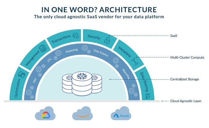
Figure 1: Snowflake architecture diagram 

Source: Snowflake presentation, The Data Platform Built for the Cloud

Some of the key innovations that leverage Snowflake’s architecture are listed below:

• Centralized, scale-out storage that expands and contracts automatically.
• Independent compute clusters that can read/write at the same time and resize instantly. Data storage is separate from compute, allowing pay-per-use pricing.
• Minimal management and table optimization. Snowflake manages all the tuning required to optimize queries, like indexing and partitioning.
• Database engine that natively handles both semi-structured and structured databases without sacrificing performance and flexibility.

Snowflake’s pricing model consists of the following elements:

• Snowflake edition and region: When you create an account you can choose between different editions that include different services; a more detailed explanation can be found here. You also have to choose the region and cloud provider where you want Snowflake to run. Depending on the edition, region and cloud platform, the price of the credit changes. It is important to note that the multi-cluster functionality is only available with the Enterprise edition.
• Warehouse size and usage per hour: Snowflake charges credits per each minute of execution time. Then, depending on the cluster size, you will be charged more credits for the same execution time as the size of the warehouse increases. The different warehouse sizes and credit usages are shown here:

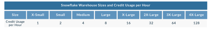
Figure 2: Snowflake’s pricing model

• Storage: fixed price of $40 per TB per month, which can get lower depending on contract conditions with Snowflake.

4. The environment

To properly benchmark Snowflake’s technology, we have to take into account ShopNow’s current stack. They have three main data sources that are processed with different Amazon Web Services to create a final star schema in their Redshift data warehouse. The main data sources are:

• User navigation in web and app: this data source is processed in real time.
• Relational Data Sources: orders, product inventory, financial data, etc.
• Third-party data sources from external tools and APIs.

As mentioned, the main compute resource of the ETL is Amazon Redshift Data Warehouse; more specifically, they were using 4 nodes of dc2.large, running 24/7 but executing jobs only 50% of the time.

To simulate ShopNow’s ETL in Snowflake, we chose to re-create their largest fact table and then estimate the cost of this part of the workflow in Redshift for comparison. This table consists of the product orders done through their platform and has a size of 6 million rows (1.5 GB). It is full loaded 6 times a day from 30 staging tables that we will use as data sources.

5. Benchmark definition

In order to achieve the goals described in section 2, we defined the following benchmarks:

• Benchmark I: Translation
  • Replicate the loading and transformation scripts that generate the largest fact table of ShopNow, which contains the orders of the different products sold on the webpage.
• Benchmark II: ETL Performance
  • Run the stored procedures that generate the fact table in Snowflake’s environment with different cluster sizes and compare it with the execution time in Redshift.
• Benchmark III: Data Visualization
  • Run a set of standard reporting queries including groups, sorts and aggregates on the fact table generated by the ETL.
• Benchmark IV: Separation of ingestion and consumption
  • Execute business user queries from simulating reporting tools while ingestion of new data is taking place.
  • Test the performance of parallel executions to verify the multi-cluster feature that allows handling concurrency.
• Benchmark V: Cost Estimation and Forecast
  • Cost estimation of the ETL and reporting queries.

6. Results

6.1. Benchmark I: Translation

As mentioned before, Snowflake and Redshift both support a very similar dialect of ANSI-SQL, and Snowflake, for the most part, supports a superset of the functionality that’s included in Redshift. But when you attempt to migrate any SQL script from running on Redshift to running on Snowflake, you’ll come across plenty of unanticipated language inconsistencies.

In this section, we’ll provide some notes on the discrepancies between both dialects that can have a larger impact on your workload. In general, the gap between the two SQL dialects has improved a lot over the past months, and our hope is that it will continue to close over time. And rest assured: if you make it through this transition process, the benefits are quite significant.

These are the SQL inconsistencies that we found when transitioning from Redshift to Snowflake, starting in order with biggest impact:

• Date and timestamp math: Snowflake does not support Postgres-style timestamp math, which Redshift does. Redshift also supports standard timestamp math, like Snowflake, but rewriting all of your date math can be a headache if you use a lot of Postgres-style syntax.

• Dealing with time zones: The Redshift approach to time zones is quite straightforward and is inherited directly from Postgres; either a timestamp has a time zone associated with it or it doesn’t. In Snowflake, things get more complicated: there are actually three timestamp formats instead of two: TIMESTAMP_NT (no time zone), TIMESTAMP_TZ (with time zone), and TIMESTAMP_LTZ (local time zone). Rather than attempting to explain all this, feel free to read the docs. Our recommendation here would be to convert all of the timestamps in your ingested data to UTC and store them as TIMESTAMP_NTZ, then let your BI layer deal with any timestamp conversions as the data gets presented.

• Casing and quotes: Snowflake handles case sensitivity very differently from Redshift or Postgres. When identifiers (table, schema or database names) aren’t quoted, Redshift will downcase them by default. So, for example, if we run these 3 statements in Redshift:

-- REDSHIFT
create table test_table as select ...;

select * from test_table;
--works
select * from "test_table";
--works
select * from "TEST_TABLE";
--fails

Snowflake, on the other hand, upcases unquoted identifiers. This leads to some very odd behaviour, and means that you need to be very careful about quoting:

-- SNOWFLAKE
create table test_table as select ...; 

select * from test_table;
--works
select * from "TEST_TABLE";
--works
select * from "test_table";
--fails 

In other databases, you can get away with using quoting loosely, but in Snowflake you must be really deliberate about what you do and don’t quote. Our general recommendation is to quote as little as possible in Snowflake, since it can be annoying to have to type out your identifiers all in caps.

• Data type conversions: A pretty common situation that occurs when you have heterogenous data sources is having two different data sources define the same column with slightly different timestamp formats, for example, HH24 and HH12 AM. Redshift sees both formats in the same column and converts both values to the same timestamp format. When Snowflake sees the same, it throws an error. This is part of a trend we can see in Snowflake: functions are less forgiving than in Redshift. The problem mentioned with timestamp conversions will force you to write regular expressions that check the timestamp format, and then it applies a specific conversion format string based on what it sees. The same occurs when converting to numeric data types as well.

• Assigning column names in DDL: Snowflake requires you to explicitly name all columns when you are creating tables and views. Often Redshift DDL can provide default column names for you. Make sure all of your columns are explicitly named in your DDL scripts.

• Specific functions and statements: During the translation to Snowflake you will encounter several functions that exist in both dialects but have different syntaxes. These cases are easy to find in the Snowflake documentation, but you will have to manually change them in your scripts. Some of the examples in Redshift are: DATE(), MONTHS_BETWEEN(), LEN() and UDF variables. The syntax to define primary keys changes and needs to be modified in your DDL scripts as well.

• Statements that don’t exist in Snowflake: As mentioned before, Snowflake manages all the tuning required to optimize queries like indexing and partitioning. For this reason, some statements in Redshift that are used to tune the database performance must be removed. Some examples are: ENCODE, DISTKEY, and SORTKEY. Our recommendation in this case is to use regular expressions to comment out these key words in all your scripts at once.

6.2. Benchmark II: ETL performance

To simulate ShopNow’s ETL in Snowflake, we chose to re-create their largest fact table and then estimate the cost of this part of the workflow in Redshift for comparison. This table consists of the product orders done through their platform and has a size of 6 million rows (1.5 GB). It is full loaded 6 times a day from 30 staging tables that we will use as data sources.

The first step was to load the 30 staging tables to Snowflake. We prepared an S3 bucket where we copied those tables and loaded them to 30 tables in Snowflake. Note that the full ETL was not completely replicated, but only the second part. The first part of the original ETL consists of copying the origin data sources into a data lake and cleaning the raw tables into staging tables; these staging tables that were already processed are the ones we used as origin to re-create the fact table. Finally, we simulated a scenario where the fact table grows to 10 times its current size to benchmark Snowflake’s capabilities in this situation.

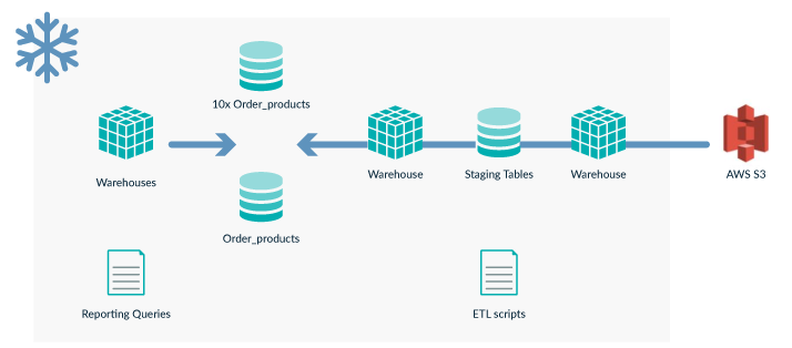
Figure 3: ETL diagram in Snowflake’s platform

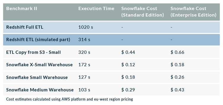
In the following table you can see the results of the tests. ShopNow’s full ETL execution time is 1020 seconds, but the part we replicated from the staging tables to the final fact product took 314 seconds of processing. The same procedure was replicated in Snowflake using 3 warehouse sizes: X-Small, Small (double the size of X-Small) and Medium (double the size of Small):

In the following chart we show the time vs the cost of running the ETL in each cluster (XS, S and M):

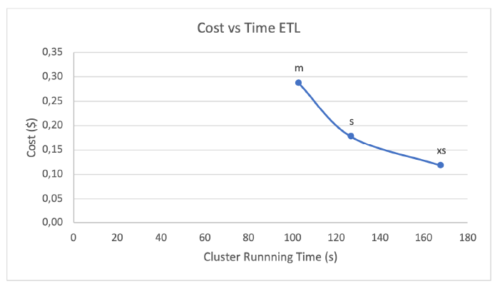
Figure 4: Cost vs Execution Time of running ETL in different warehouses

Theoretically, one should expect that running the same procedure in a cluster 2 times larger should cut the time in half, and as consequence, cost should remain the same. Visually, we could expect to see a horizontal line in this chart, where cost remains constant as we cut the execution time in half at each re-sizing. However, we don’t see this behaviour in this test because doubling the size of the cluster doesn’t reduce the execution time accordingly. Therefore, cost goes up as we use larger clusters, but execution time doesn’t decrease proportionally.

To explain this behaviour, we should bear in mind that we are running ETL scripts in this test with DDLs that create the tables and then INSERT statements that combine the staging tables into temporal tables first, which are then combined into the fact table. There is a point where having a larger cluster doesn’t parallelize the process any further and, in consequence, you don’t get the benefits of upscaling.

In Benchmark III we can observe different behaviour with the reporting queries from visualizations tools, where upscaling leverages the benefits of parallelization and we can get faster response times at the same cost.

6.3. Benchmark III: Data Visualization

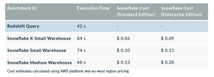
In this third benchmark, we ran a set of reporting queries including groups, sorts and aggregates on ShopNow’s fact table and the augmented fact table (10 times larger). The following table contains the results of one of the queries which aggregated the 6 million rows into 71 rows and had the most complex calculations in it:

In the following chart we show the time vs the cost of running the reporting query in each cluster (XS, S and M):

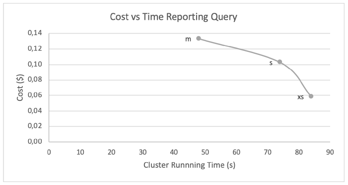
Figure 5: Cost vs Execution time of running a reporting query from visualization tool using different warehouses

One important condition to bear in mind if you want to do you own benchmark of Snowflake is to disable the cache during your tests. Snowflake stores the results of the last and most common queries in its cache to get faster response times, which would distort the comparison with Redshift.

The results of this test are similar to the ETL execution test. We should expect that running the same query in a cluster 2 times larger would reduce the time by half. However, we don’t see this behaviour in this test because doubling the size of the cluster is not reducing the execution time by half. But we can see differences when we run the queries against larger tables, where Snowflake can optimize the parallelization of the execution and leverage a larger cluster to reduce time proportionally. In the following table, we see the results of running the same query against the 10 times larger table (60 million rows and 15GB):

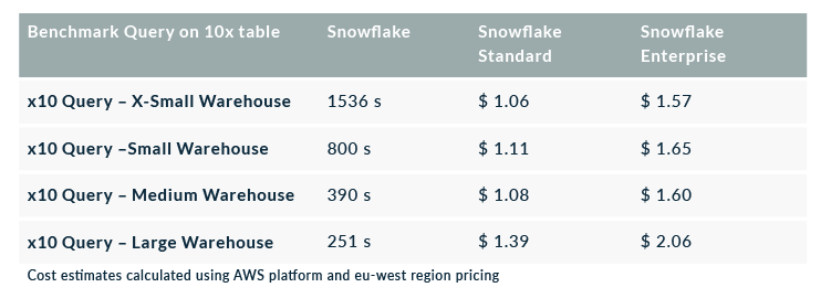
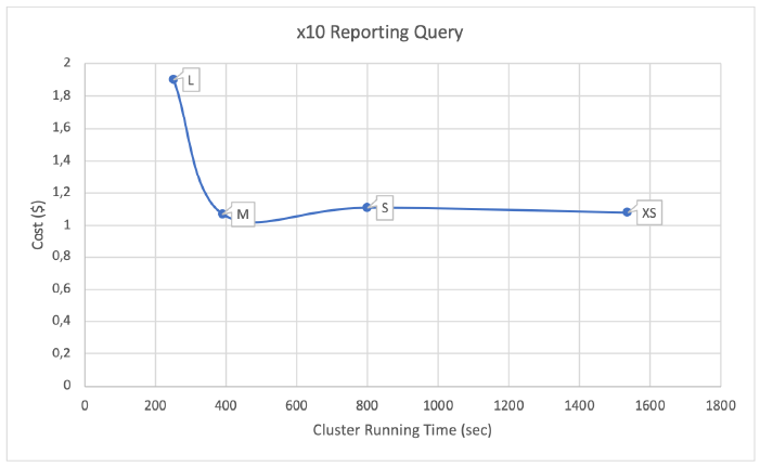
Figure 6: Cost vs Execution time of running reporting query using different warehouses (augmented x10 table)

The results presented in this chart are probably the most interesting part of this benchmark. When we run the same query against a 60 million row table instead of the 6 million row one, we observe how Snowflake is able to parallelize the query as one would expect when resizing a warehouse. We start with an XS warehouse running for 1600 seconds, then, we resize it to an S warehouse (twice the size of the XS) and we observe an execution time of 800 seconds. In consequence, the cost is now the same as before because we reduce the time by half but price doubles. The same behaviour happens when resizing to an M warehouse. However, if we keep resizing the warehouse we will get to a point where further parallelization of the query is not possible and execution time doesn’t get reduced, raising cost by more than 80%.

As you can imagine, if you decide to migrate to Snowflake, finding these ‘sweet spots’ where execution time can be reduced 4 times while keeping the same cost becomes an important task for the IT department. The flexibility of Snowflake, where you can choose to use a different warehouse for every process, plus its pay-per-use model, gives a lot of freedom to create new types of architectures. On the other hand, correctly sizing your warehouses becomes a really important task that will allow you to execute the jobs in less time with a similar cost. As we have seen with our tests, if we chose a large warehouse, we could see our cost increase by 80% without seeing a significant improvement in execution time.

6.4. Benchmark IV: Separation of ingestion and consumption

The use of several simultaneous compute warehouses in Snowflake allows for complete separation of ingestion and consumption, ensuring no process can disturb another. To test the multi-cluster functionality, we executed business user queries from reporting tools at the same time as executing the ETL. Our goal was to verify if there is any impact on performance on either side. The following table summarizes the results of 4 different tests we performed with different types of situations where concurrency could occur:

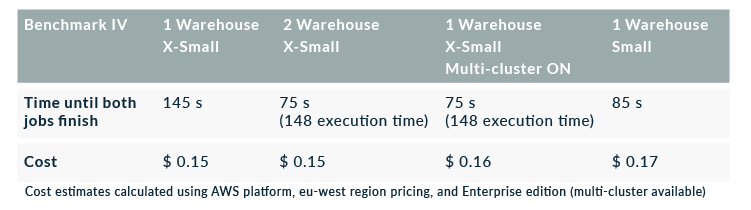
• 1 warehouse of size XS: we simulate a situation where we only have one cluster and two jobs are being executed at the same time.
• 2 warehouses of size XS: we have two warehouses of the same size, one dedicated to each type of job (ETL and reporting, for example).
• 1 warehouse XS with multi-cluster activated: multi-cluster option (only available in Enterprise edition!) allows a warehouse to auto-scale when there are concurrent workloads. In our case, we configured the warehouse to a maximum of 2 clusters.

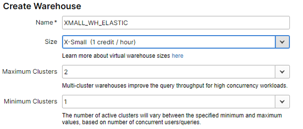
Figure 7: Snowflake’s warehouse configuration

• 1 warehouse of size S: we simulate a situation where we decide to scale up, instead of scaling out for concurrency and configure a warehouse 2 times larger than the XS.

The results are clear on which is the best option when dealing with concurrent workloads: either separate the jobs in different clusters or have the multi-cluster option activated. If you execute several jobs in parallel in the same cluster, execution time and cost get impacted. On the other hand, using separate clusters gives the same results as the multi-cluster option if you don’t have the Enterprise edition available. However, you would need to predict these concurrent workloads to create the right setup; having the multi-cluster option simplifies the architecture and administration workload.

6.5. Benchmark V: Cost Estimation

As mentioned in Benchmark I, we used 30 staging tables as our origin data source to create the largest fact table in the company. Although it is one of the critical parts of ShopNow’s ETL, it is not everything. Therefore, instead of trying to extrapolate the results obtained in Snowflake to try to obtain an estimation of the cost for the whole pipeline, we thought it would be more accurate to compare the cost between Redshift and Snowflake taking into account only the part that we simulated.

We measured the execution time of the part of the ETL that we tested in Redshift and estimated the part of the total monthly cost that it represented. Bear in mind that Redshift pricing is fixed and monthly, very different from Snowflake’s pay-per-use model where you can calculate the cost of a single query if you know the execution time.

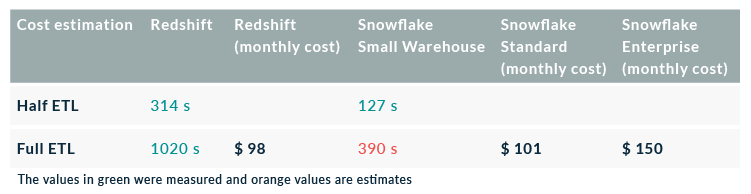
We executed the part of ETL that generated the fact table in Redshift resulting in 314 seconds (while nothing else was being executed), and we knew that the full ETL considering the creation of the staging tables took 1020 seconds. In Snowflake, we had tested one part of the ETL (using the staging tables as origins), so we extrapolated the results to estimate the total time that the ETL would take in Snowflake: about 390 seconds.

The cost in Redshift is estimated as follows:

• 1020 s x 6 times/day = 85 minutes per day
• Total Redshift running daily time: 750 minutes
• 4 nodes of dc2.large price: $ 864
• 85 minutes of ETL out of the 750 total daily minutes = 11.3 % of the time
• 3 % of $864 = $98 / month

The cost in Snowflake is estimated as follows:

• 390 s x 6 times/day = 39 minutes per day x 30 days = 1170 minutes / month
• 1170 minutes = 19.5 hours = 19.5 credits
  • Small x 2 (factor for warehouse size) = 40 credits
• Standard Edition: 40 credits x $2.5 / credit = $101 / month
• Enterprise Edition: 40 credits x $3.70 / credit = $150 / month

Finally, the following table estimates the cost of the full ETL for the different warehouse sizes and account editions:

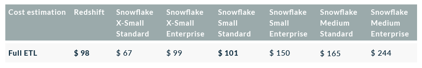
The decision to migrate to Snowflake might be for many reasons other than cost, but it is something that always needs to be taken into account. The cost estimation of the full ETL using the Standard version of Snowflake is similar to Redshift, but it cuts the execution time in half.

7. Integration with other services

Snowflake works with a wide array of tools and technologies, enabling you to access data stored in Snowflake through an extensive network of connectors, drivers, programming languages, including:

• Business Intelligence tools such as Tableau, Power BI, Qlik, etc.
• ETL tools such as Talend, Informatica, Matillion, etc.
• Advanced Analytics platforms such as Databricks or DataIku.
• SQL Development such as DBeaver or SnowSQL.
• Programmatic interfaces such as Python, .NET, node.js, JDBC, ODBC, etc.

We have tested connecting Snowflake with many of the mentioned technologies and the results have always been successful, and in some cases exceeded our expectations.

Conclusion

In this blog article we have explored Snowflake, a new data warehousing platform that has been gaining traction over the past months. We have learned some of the points to focus our attention on when considering a migration from Redshift to Snowflake. Finally, these are the important takeaways for you:

• Don’t underestimate the workload of translating your existing SQL to Snowflake’s dialect.
• Correctly sizing the warehouses will allow you to execute the jobs in less time at a similar cost.
• Our cost estimation of the Full ETL using the Standard version of Snowflake is similar to Redshift but takes half the execution time.
• When it comes to executing parallel queries, multi-clusters provide better performance at the same cost, while maintaining a simple set-up.

For more information on how to deal with and get the most out of Snowflake, and thus obtain deeper insights into your business, don’t hesitate to contact us! We will be happy to discuss your situation and orient you towards the best approach for your specific case.