28 Ene 2019 Big Data made easy

Article 3: Working with Arcadia Data to create interactive dashboards natively with a Cloudera cluster

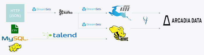
This is third part of our blog series called Big Data made easy, where we explore a set of tools that facilitate Big Data operations. For the three articles in the series we have used data from CitiBike NYC, a bike-sharing service operating in New York that chose to make their data public online. There are two types of data sources: first, the anonymized historical data of all the trips from 2013 to 2017, and second, the real-time data feed provided via a HTTP REST API that delivers JSON files with information about the current status of each station, their parking docks, the number of available bikes and other parameters.

In the first article we worked with Talend Open Studio for Big Data to load the historical data into Hive tables in Cloudera and we used Zoomdata to visualize it. In the second article, we tested StreamSets to load the data from the HTTP feed into Kudu tables in the same Cloudera cluster. In this, the third article, we’ll explain how we used Arcadia Data to visualize the data, both the historical data ingested with Talend and the real-time data ingested with StreamSets.

As mentioned in our previous blog articles, please note that the solutions presented in this article are not intended to be complex, ultra-efficient solutions, but simple ones that give our readers an idea of the tools’ possibilities.

1. Introduction to Arcadia Data

Arcadia Data is a visualization tool that offers the advantage of native integration into a Cloudera Hadoop cluster. Arcadia Data can be added, like any other service, to a Hadoop cluster; all the data stays in the cluster, so there’s no need for data movements or duplicated security concerns.

As you would expect from a modern BI tool, we can easily create dashboards where data, charts, images or even webpages and other components can be freely organized. The dashboards created with Arcadia Data are very user-oriented, with interactive components, live filtering, and other major features for working with streaming data, like auto-refreshing values. In addition to these core features, Arcadia Data also boasts some advanced possibilities like theming features or customizing visual charts with code.

However, the most distinctive features of Arcadia Data are behind the scenes. In addition to those mentioned above regarding native integration, there is a set of features worth special mention: first, the Arcadia Enterprise Smart Acceleration provided by Analytical Views, a semantic caching mechanism that allows pre-computing and caching the results of costly SQL operations, such as grouping and aggregation; second, its real-time analytics capabilities that can, for example, create visualizations directly on Kafka topics; third, its data-blending capabilities that allow data to be mixed from sources outside the cluster; and finally, the chance to reuse the Arcadia Smart Acceleration data with other BI tools such as Tableau.

2. Solution overview

For the demonstrations presented in this article and in the rest of the series, we have deployed a 4-node Cloudera cluster in Microsoft Azure. As mentioned above, we installed Arcadia Data by adding it as a service to the Cloudera cluster; there was no need for dedicated Edge nodes.

We have created three different dashboards in Arcadia Data using three different datasets. The first dashboard analyzes all the historically-tracked bike trips. This dataset is first introduced in the first post of this series, the data comes from different sources and ends up in a Hive table with over hundred million rows. The second dashboard shows real-time data on station status as introduced in our second blog post of the series: number of available bikes, number of available docks, number of non-working docks, etc. The data originates from a HTTP REST API in Citi Bike website that delivers JSON files. The data is refreshed every 10 seconds and is stored in a Kudu table. The data source for the third dashboard is the same one than for the second dashboard, i.e. the HTTP REST API in Citi Bike website. In this case, we historify the snapshots every 15minutes with a StreamSets pipeline similarly as we presented in the second blog post. The data is stored in a Hive table.

3. Connecting to data

Arcadia Data has three distinct concepts when it comes to data management:

• The connection list, which keeps track of all the connection types that have been saved.
• The connection explorer, which indexes the different datasets and their own tables when using one specific connection.
• The datasets list, which represents the tables that have been imported into Arcadia Data.

The first step is to create a connection. Arcadia Data is flexible when it comes to connecting to sources, from MySQL to Oracle, including Amazon Redshift, Spark SQL, SQLite, etc. As we are working with both Kudu and Hive tables, we want to connect through Impala, the distributed query engine from Apache Hadoop.

We need to fill in the host, IP address, port information and any optional credentials. It is worth noting that Arcadia Data is compatible with SSL socket and Kerberos (as well as other) authentication modes under the advanced settings.

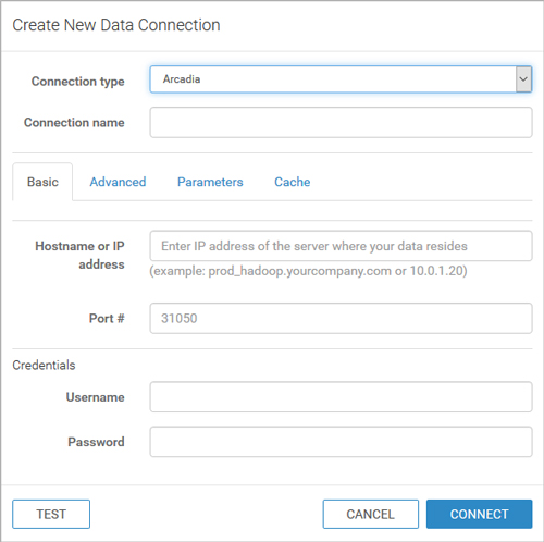
Figure 2: Creating a connection.

Once the connection has been tested and established, all the information about the workspace should be under the connection explorer. Databases and their tables should be correctly displayed, with an option for each table to create a new dataset inside Arcadia Data itself. Once we have selected the table and created the dataset, it appears under the Datasets tab, from where it can be managed.

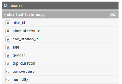
Figure 3: Fields edition.

There are several possible options now. First, it’s possible to edit the table: change the types, move fields from dimensions to measures (or vice-versa), get a glimpse of the data or join tables. There is an ‘Events’ feature, similar to the triggers in SQL, allowing us to alter columns or filter with certain conditions. Finally, we can create ‘Segments’ that can be used as filters with the ability to group a range of values (e.g. a temperature of less than -10 degrees Celsius gets the label “very cold”, which can be reused as a filter later on).

For CitiBike NYC, we used different datasets for each of our three solutions:

• First, a simple dataset composed of only the historical table for trip data from 2013 to 2017.
• For our streaming dataset, we joined three tables gathering data about station status, station information and system regions respectively.
• Finally, our historical-streaming dataset was also joined with the three datasets with the same purpose, but this time those tables were filled with the history of the older snapshots as well, as explained before.

4. Creating and organizing dashboards

At this point, the necessary datasets have been correctly imported and configured, so we can start creating and filling in the dashboards.

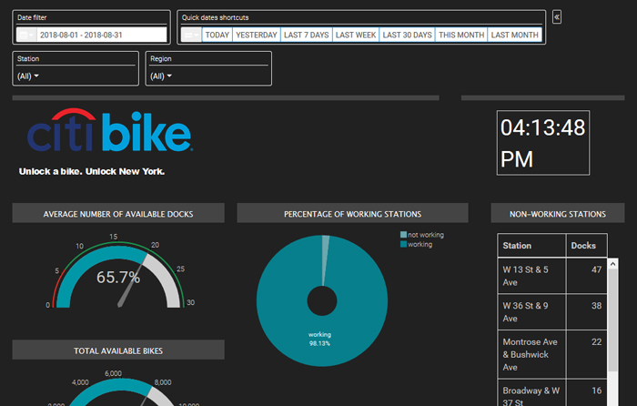
Figure 4: Example of the dashboard for the historical-streaming dataset.

Filters can be displayed at the top, bottom or at the sides of the window; it’s possible to create filters based on the fields you have. In our case the most important ones were time filters, with a calendar or with shortcuts, and geographical filters, with some information per station or for a whole region of NYC.

In Figure 5, we can see an example of the classic components as well. We can display formatted text, a frame from a webpage, or a custom JavaScript code like the clock.

For the dashboard, we chose to display important KPIs like the average number of available docks, available bikes, a list of non-working stations that need the most urgent attention, or a list of the stations with the greatest number of disabled bikes or docks.

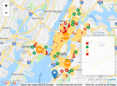
We can also use more advanced components. The interactive maps were crucial for us, and we were pleased to see that Arcadia Data comes with enough customization options to do what we wanted, like displaying a general map of the stations with their status in real time. There are two more maps, one showing the emptiest stations and the other the fullest. We know that CitiBike NYC employs more than 100 people to move bikes from one station to another, every day. Obviously, optimizing this process would create a lot of business value.

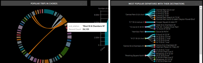
Different charts, like dendrograms or chord charts, were another important feature providing fancy visuals; they allowed us to display the most important departure and destination stations. All defined filters can be applied to these visuals.

Conclusions

While working with Arcadia Data we experienced its great user-friendly interface: we could drag and drop the columns from the data source and select the visuals we wanted to display; it was easy and intuitive. We must also emphasize the fact that it can be installed in a Cloudera cluster, so that Arcadia Data is a service in Cloudera, allowing this tool to leverage all the computing power of a Hadoop cluster. This native integration eliminates the need for a dedicated server for Arcadia Data. It has many built-in connections, from relational data sources to Hadoop ecosystem sources. The connection to Kudu allowed us to visualize real-time data capabilities.

We must also highlight some other Arcadia Data features we worked with, even though they have not been presented in this article. For instance, the coherent cache, which caches the query results from the analytics acceleration engine in memory: queries that exactly match results data in the coherent cache will automatically use those cached results; if no exact cached results exist, then the queries are checked against existing analytical views. Analytical views pre-compute the most expensive types of operations in a known workload, so you can get faster responses on sets of similar, but not identical, queries. Another feature we want to mention is “eager aggregation”; most queries in BI are star queries that operate on large amounts of data, and often run very slowly, but eager aggregation improves performance by aggregating the required data before making the joins.

Arcadia Data is one of the few visualization and BI tools aimed at Big Data; another example is Zoomdata, which we covered in the first article in this blog series. These two tools share some features, like real-time capabilities or data-blending possibilities (which can be seen as a sort of data federation or data virtualization solution). These tools are different from traditional BI tools, going beyond just exploiting the native SQL engines on Hadoop (such as Impala), with features like Analytical Views (Arcadia Data) or Data Sharpening (Zoomdata). However, data-as-a-service solutions such as AtScale or Dremio are starting to offer similar benefits to traditional BI tools, so the alternatives for visualization and BI on Big Data platforms are now more numerous than ever.

If you are wondering which architecture and set of technologies is the most suitable for your organization, don’t hesitate to contact us here at ClearPeaks – we’ll be glad to help you!