25 Nov 2021 Data Lake Querying in AWS – Optimising Data Lakes with Parquet
This article is the first in a series called ‘Data Lake Querying in AWS’, in which we are going to present various technologies for running analytical queries in data lakes in AWS.
If you are interested in building data platforms in AWS, you may also find some of our previous blogs to be of interest: in this previous article we discussed how to build a batch big data analytics platform in AWS; while in this one we discussed how to build a real-time analytics platform in AWS; finally, in another article we showed how to ingest data into AWS from any type of source and how to use an advanced orchestration service.
Coming back to querying AWS data lakes, there are many technologies out there that you can use to query big data in AWS, each with its pros and cons. We do not intend to cover all of them: in this series we will be talking about native AWS technologies, which are Athena and Redshift, as well as Snowflake, Databricks, and Dremio. We could also add Cloudera to the list, but we have already discussed Cloudera in other blog posts, so we will put it to one side in this article.
Please note that this blog series is not intended to be a comparison of these technologies, but to help you with the first steps you might take with them, showing you how to load and query data using a known and common dataset and a known and common set of queries. If you have any doubts about which tech is the most suitable for your case, please contact us and we will be happy to help and guide you along your journey.
But before looking at the various options available to query data lakes in AWS, we want to scope this initial blog article into discussing an important topic regarding data lakes, which is the format and optimisation mechanisms used in them, especially when the data is going to be used for analytical purposes; the scope of this blog is to discuss data lake formats and optimisation mechanisms.
We will also introduce the concept of the data lakehouse, which is gaining some serious momentum and is very much related to the idea of optimising data lakes for querying. Finally, we will present an example of how to apply a common data lake optimisation approach in AWS; more precisely, we will show you an example of how to transform a dataset in CSV format into Apache Parquet format in AWS, and how to partition it. These versions of the dataset, the CSV and the Parquet (unpartitioned and partitioned), will be used as a starting point in future blogs where we will look into how to use these different techs to query data lakes.
Data Lake Optimisations
Data lakes are used to store large and varied data coming from multiple data sources. Many of these data sources generate data in raw formats, such as CSV or JSON. However, using such raw formats for analytical purposes, when data gets relatively large, yields poor results. While it is technically possible to use the raw formats directly for analytical purposes, a common approach to performing in-lake data analysis is to transform the data into a format such as Parquet, which is more performant.
Apache Parquet
Apache Parquet is an open-source file format that stores data in a columnar format, compressible using efficient encoding schemes, and stores metadata in a header. These various mechanisms give much better reading performances compared to using raw formats, which is critical when using the data for analytical purposes. Moreover, a Parquet file is around a third the size of a CSV file, which saves storage costs and reduces the amount of data read, making reading Parquets much faster than raw formats.
Partitioning
In addition to using optimised file formats like Parquet, another common approach for further optimisation is to partition the data (data is stored in different folders based on a column value – or multiple columns) which will allow partition pruning when querying the data.
Basically, the folders are stored in order, so the querying engine (whatever it is) reads the name of the folder to know if the values correspond to the desired ones. This way only the wanted folders are accessed and all the content is read, while the others are skipped. Furthermore, as it is sorted, once the current value being checked is greater than the desired maximum value, the process finishes.
Alternative Formats and Optimisation Mechanisms
Note there are other formats (ORC, Delta, etc.) and other optimisation mechanisms that can be applied (clustering, for instance) instead of, or complementary to, Parquet and partitioning. Do not hesitate to contact us to discuss which combination is the best for your case.
Data Lakehouses
And while we are on the subject of data lake optimisation for querying, we should mention a trending concept: data lakehouses. As the name suggests, this concept, or umbrella term, defines a platform that combines the storage reach of the data lake (store all you want) with the analytical power of the data warehouse (query all you want).
Sadly, as is often the case with buzzwords, there does not seem to be a common definition of exactly what a data lakehouse is, since each vendor has their own definition (usually highlighting the aspects in which each tech shines). Check the definitions of the different techs we will cover in this series: AWS, Snowflake, Databricks and Dremio, and you will see the broad spectrum of definitions of this new buzzword.
Data Lake Optimisation Example
Now that we are done with the introductions, in the following sections we are going to demonstrate how we can optimise a data lake via an example dataset. We will first generate the dataset in CSVs, and then convert them into Parquet without and finally with partitions, thus ending up with 3 different versions of the dataset.
Example Dataset
The dataset we are going to use in this blog series is the famous TPC-H benchmark dataset. This dataset is composed of 8 tables and emulates any industry which sells or distributes a product worldwide, storing data about customers, orders, suppliers, etc. You can see the data model below:
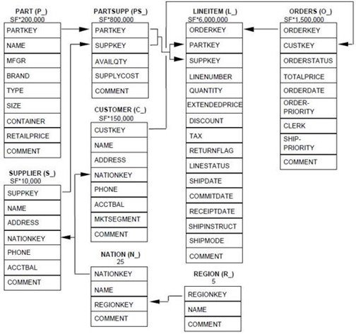
The numbers below the table names represent the number of rows in each table in a proportional way. We can see that lineitem and orders are quite large tables in comparison to others, such as region or nation.
In this article, we are going to generate 3 different versions of the same dataset in different formats, first generating the raw data (CSV), and later converting it into Parquet files without and finally with partitions (only the largest tables – lineitem and orders). In the following sections we will explain how we generated the raw data and the unpartitioned and partitioned Parquet files.
In the next blog posts in this series, we will use various data lake querying engines to query the 3 versions of the dataset, and we are going to connect a reporting tool such as Tableau to each engine to perform some operations too – to be specific, we are going to perform 10 queries from the official TPC-H specification document.
Generating the Dataset
The generation of the dataset was quite a simple step as we used the tool tpc-dbgen that automatically generates the dataset with 8 folders, 1 per table, with a specified number of CSVs in each. Specifically, we created a total of 100GB of CSVs, with 80 CSVs for each table to give more realism (the small tables, such as nation, only have a single file).
Converting CSV to Parquet and Partitioning the Dataset
Once all the CSVs have been placed in the S3 bucket, there are two different AWS services to convert them into Parquet:
Both services have their pros and cons, and we will explain them below:
Athena
The first option we are going to explain is the cheapest and fastest to create Parquet files. Athena is a serverless query service with no administration required that allows users to query data from multiple AWS services such as S3, and you are billed for the amount of data scanned. It is also possible to create databases (table containers) and tables using Glue Data Catalogs, which is free of charge as Athena is not billing DDL statements. Check Athena pricing for further details. Bear in mind that you can store up to one million objects in Glue Data Catalog for free – see the Glue pricing page.
As well as regular queries, we can also create tables from query results (CTAS). This functionality allows running a statement to create Parquet files from CSVs and also automatically creates its Data Catalog table.
First, to read the CSV, we had to create a Data Catalog pointing to each table folder in S3. We first created a database and all the tables, but for simplicity’s sake we will only show the orders table. Although you could create the table and the database directly in the Glue Data Catalog page, we ran this code manually in Athena:
CREATE database IF NOT EXISTS tpc_csv;
CREATE external TABLE tpc_csv.orders(
	o_orderkey BIGINT,
	o_custkey BIGINT,
    	o_orderstatus varchar(1),
	o_totalprice float,
	o_orderdate date,
	o_orderpriority varchar(15),
	o_clerk varchar(15),
    	o_shippriority int,
	o_comment varchar(79)
)
ROW FORMAT DELIMITED
FIELDS TERMINATED BY '|'
STORED AS textfile
LOCATION 's3://your_s3_bucket/tpc-h-csv/orders/';
Basically, we defined each attribute type, indicated the location in S3 and specified the separator, which is ‘|’. This is because dbgen generates TSVs, not CSVs, but there is no difference except the separator.
Once all the tables had been created in the Catalog, the SELECT AS statement can easily create the Parquet file without partitions.
CREATE database IF NOT EXISTS tpc_Parquet;
CREATE TABLE tpc_Parquet.orders
WITH (
	format = 'Parquet',
	Parquet_compression = 'SNAPPY',
    	external_location = 's3://your_s3_bucket/tpc-h-Parquet/orders/'
) AS SELECT * FROM tpc_csv.orders;
As you can see, with a few lines of code, we have created the Parquet files in S3 and also the Data Catalog table orders in the database tpc_Parquet from the result of selecting everything from the tpc_csv database.
Partitioning with Athena
As discussed above, although converting to Parquet is a great improvement for querying, it is also possible to further optimise it by partitioning the data, enabling pruning of unnecessary data when queries are run. Note that partitioning only really makes sense for large tables. The key, of course, is to select proper partitioning columns.
In our case, we looked at the queries defined in the TPC-H specification and easily identified the column l_shipdate from the lineitem table and the column o_orderadate from orders as the most suitable partitioning columns. Essentially, we looked at which columns were more often found in the filtering statements of the queries; once the partitioning column has been identified, the code to create a partitioned table from another table is (example shown only for the orders table):
CREATE TABLE tpc_Parquet.orders
WITH (
	format = 'Parquet',
	Parquet_compression = 'SNAPPY',
    	partitioned_by = ARRAY['o_orderdate'],
        external_location = 's3://your_s3_bucket/tpc-h-Parquet/orders/'
) AS SELECT * FROM tpc_csv.orders;
Notice the ARRAY in the partitioned_by, which is mandatory even if you are using a single partition key. After creating the partitioned table, it will not yet be queryable until you run the command to scan the file system for Hive compatible partitions:
MSCK REPAIR TABLE tpc_Parquet.orders
Nonetheless, Athena CTAS has a limitation: it can only create a maximum of 100 partitions per query. In our case it is a huge limitation because we have 8 years’ worth of daily data, and we want to partition by date on a day level.
Having said that, there is a workaround explained in the AWS documentation using INSERT INTO to “append” the partitions. However, this option might need the development of a script to automate and ease the process, which can be tedious. It might be a good idea to consider Glue for creating Parquets with more than 100 partitions in a single execution.
Glue
AWS Glue is a serverless ETL service where you can build catalogues, transform and load data using Spark jobs (PySpark, specifically). It also provides a framework on top of Spark called GlueContext that simplifies job development. What’s more, AWS has recently incorporated Glue Studio, a UI to create Glue jobs without coding by dragging and dropping boxes to apply a few configurations. Glue Studio automatically creates GlueContext code from the visual flow, and you can review it before executing.
So, we used Glue and Glue Studio to convert our CSV into Parquet and to do the partitioning; while we eventually succeeded, we encountered some issues that we will describe below in order to help others attempting the same.
We first tried Glue Studio reading directly from S3, rather than from the catalogues. However, none of the decimal values could be read; all were set to null or blank. This was fixed when we changed to using the catalogue as source, though we also had to switch to regular Glue jobs and edit the ApplyMapping where we could cast floats into decimal (this is required due to decimal being the default floating data type in Parquet). Finally, we attempted to write and partition the data by properly configuring the write_dynamic_frame function of the GlueContext:
datasource = glueContext.create_dynamic_frame.from_catalog(database =
"tpc_csv", table_name = "orders", transformation_ctx = "datasource")

applymapping = ApplyMapping.apply(frame = datasource, mappings = [("o_orderkey", "long",
"o_orderkey", "long"), ("o_custkey", "long", "o_custkey", "long"), ("o_orderstatus", "string",
"o_orderstatus", "string"), ("o_totalprice", "float", "o_totalprice", "decimal"),
("o_orderdate", "date", "o_orderdate", "date"), ("o_orderpriority", "string",
"o_orderpriority", "string"), ("o_clerk", "string", "o_clerk", "string"),
("o_shippriority", "int", "o_shippriority", "int"), ("o_comment", "string", "o_comment",
"string")], transformation_ctx = "applymapping")

datasink = glueContext.write_dynamic_frame.from_options(frame = applymapping, connection_type
= "s3", connection_options = {"path": " s3://your_s3_bucket/tpc-h-Parquet/orders" ,
"partitionKeys": ["o_orderdate"]}, format = "Parquet", transformation_ctx = "datasink")
Nonetheless, all the partitions were being created as __HIVE_DEFAULT_PARTITION__, which means that the field used to partition is null. On investigating, we realised that the class ApplyMapping, which is used to select the columns you want to use, rename columns, and for type casting, was converting all the date values to null when we were only selecting the fields without any specific mapping (casting into the same column name and type).
To fix this, we had to use the standard PySpark DataFrame and its operations. The code we used is:
datasource = glueContext.create_dynamic_frame.from_catalog (database =
"tpc_csv", table_name = "orders", transformation_ctx = "datasource")
df = datasource.toDF()
df = df.drop("col9")
df = df.withColumn("o_totalprice", col("o_totalprice").cast(DecimalType(18,2)))
df.show(10)
df.repartition(1,col("o_orderdate")).write.Parquet(s3://your_s3_bucket/tpc-h-
Parquet/orders', partitionBy=['o_orderdate'])
We used GlueContext to read from the catalogue and then converted the Glue DynamicFrame into a PySpark DataFrame; then we dropped an extra column and casted a decimal field to DecimalType, because Parquet native type for decimal numbers is Decimal. Lastly, when writing the Parquet files to S3 from the DataFrame, we set the repartition to 1 because the amount of data generated each day is not over 100MB, so it is faster to store everything in a single file, and also faster to read.
Note that we only partitioned the largest tables (orders and lineitem).
Coming Next
With the approach discussed above, we successfully created these three different versions of the same TPC-H dataset:
- Raw: CSV data generated with the tpch-dbgen tool. The raw version of the dataset is 100 GB and the largest tables (lineitem is 76GB and orders is 16GB) are split in 80 files.
- Parquets without partitions: CSVs are converted to Parquets with Athena CTAS. This version of the dataset is 31.5 GB and the largest tables (lineitem is 21GB and orders is 4.5GB) are also split in 80 files.
- Partitioned Parquets: the largest tables – lineitem and orders – are partitioned by date columns with Glue; the rest of the tables are left unpartitioned. This version of the dataset is 32.5 GB and the largest tables, which are partitioned (lineitem is 21.5GB and orders is 5GB), have one partition per day; each partition has one file. There around 2,000 partitions for each table.
These 3 versions of the same dataset are going to be used in our coming blogs. Stay tuned!
Conclusion
In this blog we have discussed how to optimise data lakes by using Parquets and optimisation mechanisms such as partitioning. We have also introduced the concept of the data lakehouse, a buzzword hitting the market now and based on the idea of querying data lakes by conceptually combining them with data warehouses.
We have also demonstrated how to convert CSVs into partitioned Parquets in AWS. We have seen that the easiest and cheapest way to create a Parquet file from a raw file, such as CSV or JSON, is using Athenas CTAS. However, when we also want to partition the data, Athena is limited to a maximum of 100 partitions; this can be solved by using multiple INSERT statements or by using a Glue job with PySpark DataFrames.
In the next blog posts in this series, we are going to use different data lake querying technologies to load and query the 3 versions of the dataset we have created here. We will then be able to assess the impact of using proper formatting for a data lake.
Here at ClearPeaks, our consultants boast a wide experience with AWS and cloud technologies, so don’t hesitate to contact us if you’d like to know more about these technologies and which would suit you best.
The blog series continues here.