07 Oct 2021 ODI Multiple Execution Units and their Advantages

In one of our customer projects, we needed to identify the part of an ODI (Oracle Data Integrator)-generated mapping query that ran for longer than expected and then fix it with the help of various options in Oracle SQL Query; but how could we do it in ODI?

One of the simplest and most effective options is to use hints or indexes. In ODI, it is only possible to apply Oracle hints or indexes on the overall SELECT at LKM (Load Knowledge Module) level, or on the final INSERT at IKM (Integration Knowledge Module) level. In these solutions, we may need to create separate DB objects in the background in order to make the query run faster.

In ODI12c, there is an option available to split the execution units in the same physical mapping layer. In this way we can separate the lines of SQL code (i.e. Sub SELECT/INLINE query) from the main pipeline, identified as a potential performance bottleneck. Splitting execution units (EUs) is not a new idea in ODI, and by default is taken care of by Groovy code while generating physical mapping. If there is only one target or the same physical/logical architecture with the same schema, then Groovy creates only one EU by sharing the same name as the target table, suffixing with _EU or simply <DataModelName>_UNIT.

If we separate the Sub-SELECT pipeline from the main flow as shown in demo example below, we can create a new EU of our own. This will allow us to bring in other EKM (Execution Knowledge Module) and LKM options to set, and also to execute the particular line of SQL code to run on a separate source or target or staging schema. Likewise, we can create N, the number of EUs in one single physical mapping. This is one of the major query optimisation features in ETL mapping performance using ODI.

Demo Example

In the following example, we have created a simple ETL flow by considering both source and target on the same database; Groovy treated it as one EU, US_ANALYTICS_UNIT, by default.

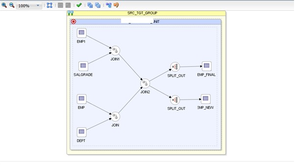
Please note that this default physical mapping won’t allow the setting of a specific LKM (i.e. C$ temp table) at source level, as all are sharing the same physical/logical architecture.

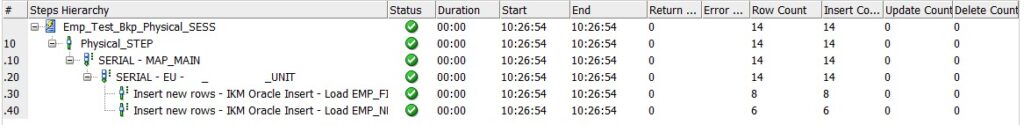
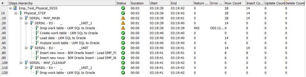
When we check the same in Session Logs under Operator, we can see only one EU created.

How to create a new EU

To make this demo use explicit LKMs or create separate EUs, we simply select the component at which point we would like to separate the flow from main pipeline and drag it outside the current execution unit so that it creates a new one automatically. Later, we can execute it in either a separate schema or just create a C$ temp work table so that we can apply the required temporary hints/indexes in LKM Options based on the LKM we use.

Before

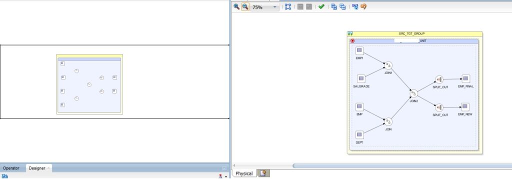
In this example, we have decided to separate the flow at the “JOIN” component, so we can do so by simply dragging it outside.

Here, we can see that the new component will be created as JOIN_AP, so when we click on this component, we can view LKM Selector and its corresponding Options in the Properties pane as shown below:

After

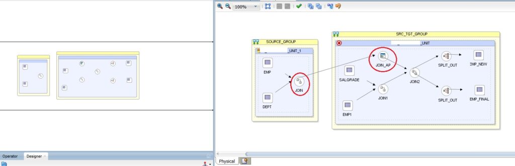
Now when we execute this mapping, we can observe a new EU suffixed as _1, as shown below:

This solution is more effective in large complex mappings, and we can clearly see the difference in performance. In this example, we created the demo with simple SCOTT schema tables and with small data.

Demo on Large Volumes of Data

Further to the above example, we will now show you a particular use case, dealing with large volumes of data based on a real project requirement. In this case, the data needs to be loaded into 2 separate targets in the logical mapping design (even though both logical targets point to the same physical table). The requirement and data integration logic is such that it requires different field criteria and insert/update logic in each of the targets.

Before the Changes

First, we tried to load a single EU as shown in the screenshot below, using default physical mapping (i.e. named Original):

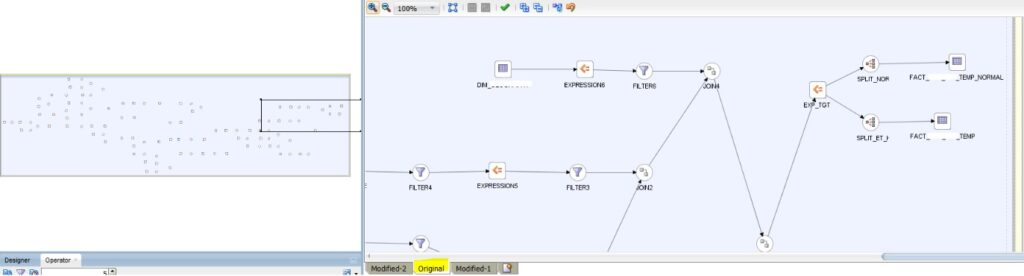
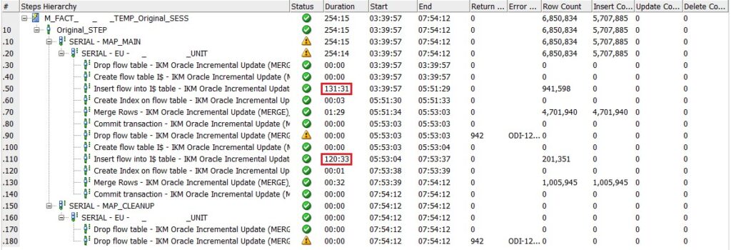
We can see where the execution time for each pipeline took more than 2 hours:

After the Changes

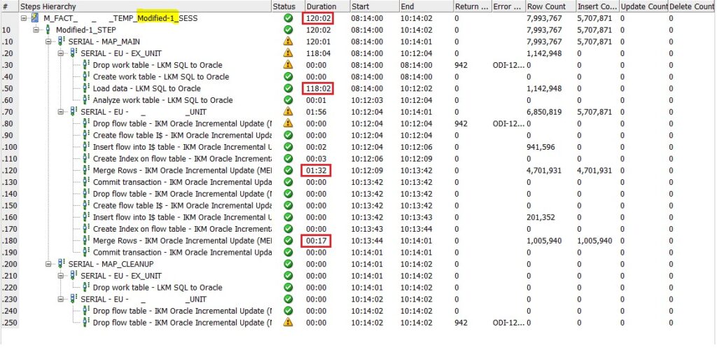
Now, after splitting the EUs as shown below at the expression EXP_TGT in the new physical mapping (named Modified-1):

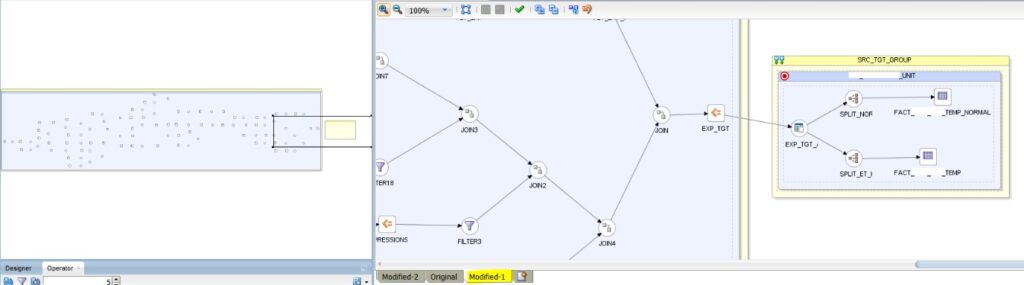
Compared with the previous run, execution time has been improved drastically, cutting the overall execution period by almost half, where the insert into the final target split has been loaded in no time at all. This example showcases how ETL performance can be twice as fast on average.

Below are the execution results after introducing the new EU:

Advantages:

• Helps to achieve faster, optimised query performance across multiple targets based on Oracle recommendations.
• Can be used to derive the inline query and fine-tune it without disturbing the main pipeline, especially in the case of reusable mappings and left outer joins. We are also consolidating the entire query in C$ and loading into multiple targets, based on requirements.
• It is easy to transform the whole reusable mapping to merge inside the main mapping with the help of these EUs, dragging them outside.

Limitations:

• Before making the changes, you must understand there won’t be any “undos” in ODI as per its basic UI design, so please ensure you have an original copy as mentioned in the point below.
• It is preferable to create a new physical mapping that will create the EU for you before you start making modifications, rather than taking a backup copy of the entire mapping.

Here at ClearPeaks this is just one of the many solutions we’ve worked on in ODI, so if you’d like to learn more about how we can speed up your BI processes, just contact us!