17 Apr 2018 Oracle Analytics Cloud (OAC)

Last year, Oracle launched the Oracle Analytics Cloud (OAC). Although it may seem that it is more of the same in terms of the data analysis tools found in Oracle Business Intelligence Cloud Service (BICS) — seen here — OAC offers a great avenue for a cloud-based BI solution that provides the benefits of low entry costs, fast implementation, and an elastic platform that can be configured in terms of CPUs and storage space.

Basically, OAC is Oracle Business Intelligence Enterprise Edition (OBIEE) running in the Oracle Cloud. The fundamental differentiations from its predecessor (BICS) are listed below, although it has to be said that BICS is currently included in OAC.

OAC:

• User managed
• Flexible licensing
• Includes Essbase
• Cloud Data Modeler or use BI Admin Tool

BICS:

• Oracle managed
• Simplified licensing
• No Essbase
• Cloud Data Modeler

OAC includes the Day by Day mobile application, which provides simple answers to daily business questions. By searching for a commercial question, the application will automatically know what you are interested in, who you share information with, and when and where that information is important to you so that you can make better fact-based decisions.

Use case

Our use case of OAC uses the Data Sync application for loading data from an on-premise schema into a schema provisioned on the Oracle Business Intelligence Cloud Service. Data Sync can be obtained from the Oracle website easily. It supports the load and merge of different relational sources in addition to Oracle, including DB2, Microsoft SQL Server or Teradata. When the application is started, the first step is to configure it and choose a password, which will always be requested the next time you access it. You will then be prompted to either create a new project or select an existing one.

Once we have access, the first step is the configuration of the connections, one against our data source and another against the cloud service. It is advisable to test the connections to make sure that they are correct and that we have access to our data and the cloud.

Figure 1: DataSync connections.

Once the connections are ready, the next step is to move into the project tab, import the tables or files (in our example we will only import tables), and define the transformations, joins, etc, that we want to apply to our tables. In our case, since the data comes from a local database, we will choose the ‘Data from Table’ option in the Relational Data tab. To collect the data directly from a query, we choose either the tables in the cloud or select ‘Data from SQL’. For the former, we choose the tables by selecting the corresponding check and pressing ‘Import’. In the case of the latter, we directly define the query that we want.

Figure 2: DataSync: import tables.

Once we have the imported tables, we choose the loading strategy that best suits each of them.

Figure 3: DataSync: load strategy.

In the Target tables/DataSets, we can see the destination tables that we have defined. By selecting each of them, we can see its details in the bottom part of the screen. We can add columns, define a default value, delete them or deactivate them.

Returning to the previous tab, we can define the joins and the transformations that we want for any source table by selecting the specified tables, and adding our definitions to the bottom of the mapping tab.

Figure 4: DataSync: toolbar where we can define joins and mapped new columns.

Unmapped columns are the new columns that we have created in the destination table and that we want to input with some kind of transformation. To do this, we have to drag them to the column on the right, as shown in the figure below.

Once added to the table, we define the transformation we want in the target expression column. In our example, one column will be informed through a lookup and another column will be an operation of two other columns. To be able to inform the field that will come from the lookup, it is necessary to first define the joins in the corresponding tab as shown in the figures below.

Figure 5: DataSync: joins definitions.

Now that we have the tables defined, the last thing that is missing is to upload the tables to the database of the cloud. For that we choose the Job tab. A Job is defined like a unit of work that can upload the data from one or more tables/files as defined in the project. By default, one is created that executes all the defined tables that are not deactivated. Press the ‘Run Job’ button and, if everything goes well, the status will display in History once finished. If on the contrary there was some error in the load, the executions of the different tasks, and their errors, are described with their corresponding logs in the lower part of the screen.

Now that we have the tables uploaded to the cloud database, we can access the OAC. Our goal here is only to define the data model with which we will make a small report in OBIEE Cloud or in Data Visualization, without the need to create the whole model step by step through the RPD. In this sense, OAC is very intuitive and makes it very simple to define the model.

First, we go to the Data tab. In the right corner we can find an icon, which if we open it, gives us the option to Manage Models.

Figure 6: OAC: Manage Models.

The Data Modeler will open and there we choose ‘Create model’. The tables that we just uploaded with the Data sync will appear in the left part of the screen in the Database tab.

Once at this point, we only have to define our facts table, our dimension tables, and our joins. An important detail is that we will always have to block the ability to modify anything in the model, the button is in the top right.

To define the tables that will be part of the model, click on the icon of each of them and choose ‘Add to Model’. Another window will open in which you can choose between Fact or Dimension.

Figure 7: OAC: tables definition to be part of the model.

To define the corresponding metrics in the fact table, we must enter the edition of the same and, as shown in the figure below, we can then choose the type of aggregation of any of the columns. We can also define hierarchies intuitively for the dimension tables.

Figure 8: OAC: metrics and hierarchies definitions.

The only thing that we need now would be to create the relationships between the fact table and dimensions. By pressing the ‘Create Join’ button, we once again can simply and efficiently create the corresponding joins.

In the following figure, you can see the general vision of the model, with the tables involved and the joins. The last thing that we need to be able to start doing reports is to unlock the edition by publishing the model.

Figure 9: OAC: created model.

Now is the time when we can access the OBIEE in the cloud or Data Visualization Cloud Service (DVCS) and do our analysis or visualization. Oracle OBIEE and Oracle DVCS are two such data visualization services that help businesses navigate the vast data analytics universe by transforming data into easy-to-understand visuals and simplifying the analytics process.

On the OAC home page, we click ‘Open Classic Home’ and open the OBIEE as we know it on-premise. When creating our report, we can see that the subject areas our model created with the Data Modeller are already available. By dragging a few objects and choosing different visualizations, we can easily create an analysis model.

Figure 10: Access to OBIEE and the subject area created.

Figure 11: Report created with OBIEE.

On the other hand, we have the DVCS, which is a web-based tool that allows simple and easy visual data analysis, even individually.

Figure 12: Report created with Data Visualization.

Oracle Analytics Admintool can connect and edit online metadata on Oracle Analytics Cloud Servers (feature available with OAC and Admintool version 12.2.2.0.30). Once repository opens, you can proceed to edit online metadata and publish changes to cloud.  Use online editing for small edits. Large edits are recommended to be done in offline mode. You can see that the model that we created in the OAC is defined perfectly in the RPD, including the tables involved, the hierarchies created, and the metrics and dimensions. Exactly everything that we model more easily in the OAC will be displayed in the RPD.

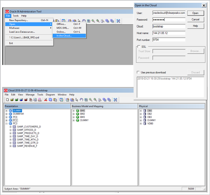
Figure 13: AdminTool: model created in the cloud.

Conclusion

So, Oracle Analytics Cloud (OAC) is a cloud-based platform with which, in a very simple and intuitive way, developers and specially end users can create their own data models. In addition, collecting information from various source systems such as Oracle DB or excel sheets themselves can join the data to obtain a more complete and fully customized analysis. A great advantage is that the user does not need to define the model through the RPD because it is a more cumbersome and more technical tool to manage than the data modeller that includes the OAC. Finally, there is no need to worry about servers, storage space or software.

Don’t hesitate to check our cloud services and  contact us if you would like to receive more information about Oracle Analytics Cloud (OAC).