10 Mar 2021 Building a Cloud Data Warehouse with BigQuery

In this article we present a solution we have recently implemented for one of our customers using Google Cloud Platform (GCP), leveraging Cloud Storage and BigQuery.

Our client is a multi-national company that has tens of Terabytes of data stored on an on-premise shared drive. The data is split by country and by month.

The aim was to build a serverless and performant Cloud Data Warehouse in which access rules per market can be applied. That is, most business users would only be allowed to access the data of their own market in read-only mode, except for some privileged users who could access the data of all markets. Moreover, a set of guard-rails mechanisms needed be put in place to keep the costs under control, since the expected number of users was very high.

Note that the characteristics of the data we described and the requirements of the solution that had to be built to deal with such data could be related to diverse business scenarios: items sold done by a multi-national retail company, CDR records of a telecommunications conglomerate, transactions of a world-wide financial institution, and pretty much any company that has multi-national coverage.

Leveraging optimisations such as partitioning, clustering, time-based views, and of course the under-the-hood columnar format used by BigQuery, we have built a Cloud Data Warehouse on GCP that many business users are already using on a daily basis for their analysis. Not only that, but we have also created a smart Python-based tool that is capable of loading tens of gigabytes every week from on-prem locations into Cloud Storage first, and finally BigQuery.

1. Achieving Country-Based Access Control with Projects, Views and IAM

So, you may be wondering how a certain user could only access the data of one country, while another user can access data from another country, and a third privileged user can access all of them. To achieve this, we combined a set of features available in BigQuery.

For those who don’t know, Google Cloud services are grouped into Projects. These projects are the basis for controlling user permissions on the services contained therein, facilitating the work of the finance department to be able to centralise, if desired, the billing accounts of all projects in the same account.

In our solution, we have created many Projects. The most important one is called “Core”. In the “Core” Project, all the data from the on-premise source systems is uploaded to Google Cloud Storage, and from there it is loaded into BigQuery. The only user with access to this Project is a service account in charge of performing the loading of the data.

In addition, a Project is created for each country, and these “country” Projects only contain read-only views that point to subsets of the data contained on the “Core” Project. Therefore, users with access to a certain “country” Project will only be have read-only access the corresponding data of that country. Finally, an “ALL” Project is created where users can access, also in read-only mode via views, all the data from the different countries. This is useful for members in the organisation that need to see aggregated data of the entire organisation.

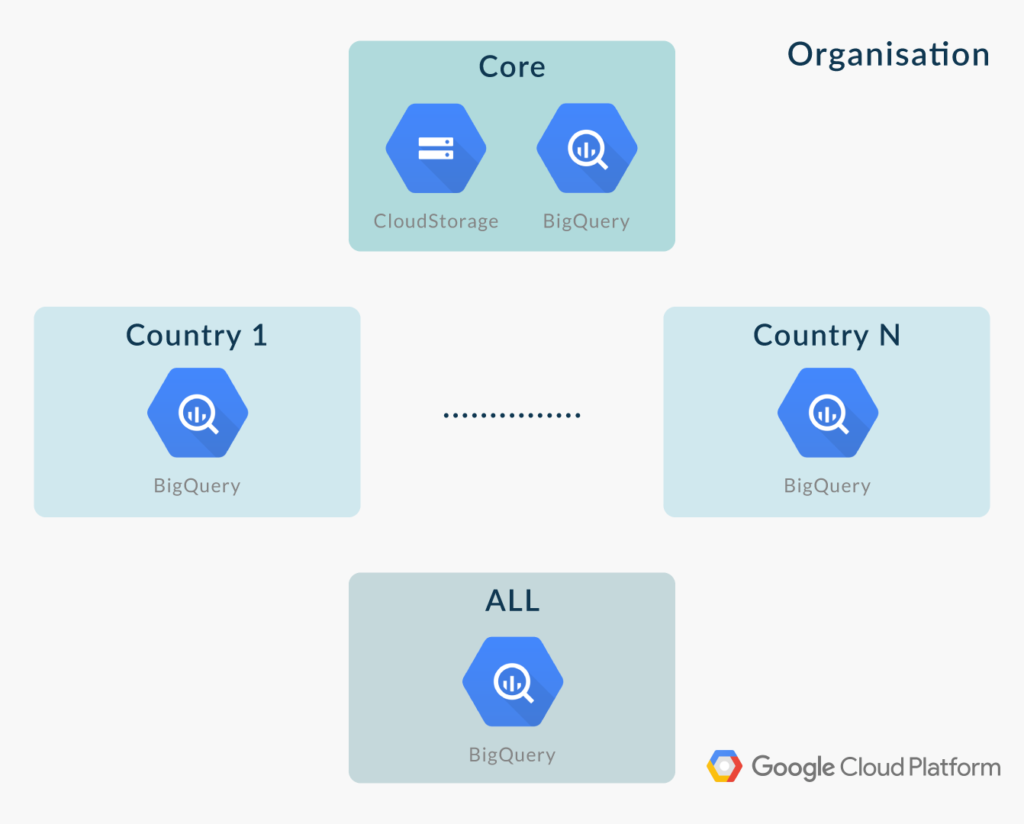
Figure 1: Projects structure

Access to the different Projects is done using Cloud Identity and Access Management (IAM), and access is granted according to the group to which the user belongs. For each Project, there are two groups, the first one is for users who perform queries on BigQuery, while the second one has the same privileges as the first one as well as access to quotas management (this is described below).

The most important thing to do in controlling the cost of BigQuery is to educate the users about how to use the platform in a cost-effective manner. We did that, of course, but we all know that that may not be enough, and it is important to put other measures in place. Essentially, we have limited the cost per user through quotas, specifically through the fields “BigQuery query limit per project per day” and “BigQuery query limit per user per project per day”.

2. Data Loading with Python

We have implemented a Python tool using the Python APIs for Google Cloud Platform, which runs on an on-premise Linux Virtual Machine (VM) and performs the whole loading process automatically.

Every week, new data becomes available on a large on-premises shared drive for all the countries. These can be ZIP or GZIP files, and each ZIP or GZIP file can contain one or more CSV files. These CSV files do not have a fixed schema. There are a set of common fields, but depending on the country and the month, the attributes contained in the files can vary.

CSV files in GZIP can be loaded into BigQuery. CSV files in ZIP cannot be loaded in BigQuery. The Python tool automatically detects when new data is added into the shared drive, and if needed, converts the files from ZIP into GZIP (using Linux pipes).

For each country, once the files of the week are in GZIP, they are uploaded in parallel to Cloud Storage in a single Bucket into the “Core” Project. Therefore, all the data is centralised and repetitions that may generate possible inconsistencies are avoided.

To minimise storage costs, we apply a policy that after one month, the stored files are changed from Standard type (more expensive storage but more accessible data) to Archive (much cheaper, but very expensive access). This is because once files are loaded in BigQuery we only want to keep them as backup, which theoretically will not be accessed again. You can find more information about storage types here.

For each country, once all the files of the week are uploaded into Cloud Storage, the Python tool creates a temporary external table that points to the files in Cloud Storage. This external table is used to ingest the data into BigQuery in the “Core” Project.

This external table is created dynamically – the Python tool determines which fields are present for this week and declares only these in the external table. The Python tool also generates the insert statement (which is used to insert the data from the external table into the final table in BigQuery) dynamically. The insert statement fills the missing fields with nulls when the data is inserted into BigQuery.

Once the data for a country in a particular week is inserted into BigQuery, the external table is automatically deleted. At this point, the data can be accessed through the market views by the business users.

The Python tool execution is scheduled using the Linux cronjob tool. Considering the amount of data that we are uploading; it might be possible that the processes overlap. Hence, to avoid this, we use the flock tool that checks if the cronjob is already running.

To have a better overall tracking, different techniques are used to control what data is uploaded and when.

• Tracking files: When the weekly data of a country is being uploaded from on-premise into Google Cloud, the path to the data in the shared drive is added into a first tracking file which tracks all the data being uploaded. Once uploaded, the entry is deleted from the first tracking file and added into a second tracking file, which registers all the data already uploaded into BigQuery. Therefore, if for any reason the upload process fails, we just need to check the last entry in the first tracking file to detect which data could not be inserted in BigQuery.
• Added fields (loading meta-data): We have added two extra fields in the BigQuery tables: one with the source file name and another with the upload date. These fields are helpful to monitor the entire loading process.

3. BigQuery Optimisations

In addition to splitting the data by country, we are also using other optimisations.

Most analyses done by business users require performing queries by date and location. Therefore, we use the partitioning and clustering capabilities of BigQuery: we partition the data by a date field, and we cluster the data by geopoint (st_geogpoint), which is a Google Geography type constructed by the fields Latitude and Longitude from the source data. This decreases the costs and improves the performance of the queries.

As mentioned above, business users access the data via read-only views. For each country, different views are created that limit the time span – one view limits to the last 3 months, another view for the following 3 months and so on. This ensures that users cannot query large time spans.

Conclusion

In this article, we have explained how to create a Cloud Data Warehouse in BigQuery that uploads on-premise data using Python. Our solution also provides advanced access controls leveraging Projects, Views and IAM.

Google Cloud is a very versatile cloud service provider with a multitude of services, such as the powerful BigQuery. Here at ClearPeaks, we are experts in cloud solutions, and we adapt perfectly to the client requirements and needs.

We hope you found the reading useful and enjoyable. Please contact us if you’d like to know more about what we can do for you.