05 May 2022 Cost Management in Google Cloud Platform

Cost management is one of the key points to take into consideration when choosing a cloud for your project. Unfortunately, tracking costs and being aware of what you are being billed for can be tricky when working in cloud environments.

In this article we are going to review Google Cloud Platform (GCP) cost management, from the basics to more advanced insights, focusing on BigQuery and Cloud Storage. These are the main services we have used in our GCP projects, presented in our previous articles: Building a Cloud Data Warehouse with BigQuery and Serverless Near Real-time Data Ingestion in BigQuery. For obvious reasons, the data displayed in this blog post isn’t from a real project, but it will still help us to get a better understanding of the following sections.

1. Google Cloud Billing

Google Cloud provides a Billing page in their portal to manage the costs of the services used. The first step to use this capability is to configure a billing account for a personal account or for an organisation account by adding a payment method. It is possible to define multiple billing accounts and assign them to different projects, which is handy when dividing costs within an organisation, for instance, across departments.

The most basic insights can be obtained from the Billing page itself, where you can access the Billing sections and see the cost of a single project or the overall cost of all the projects. In the Overview section we can find the total cost billed by Google for each month. To obtain a more detailed visualisation, Google provides a Reports section with several filters, like Group by Project if you have an organisation, or Group by Service to filter the costs of a specific service.

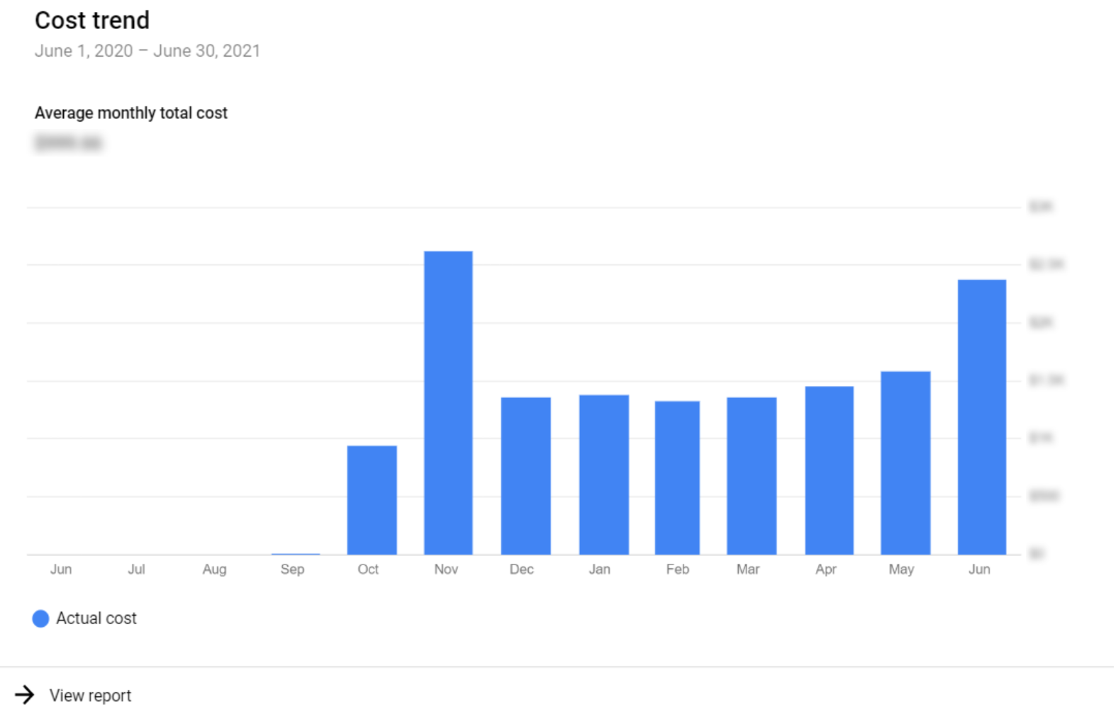
Figure 1: Organisation monthly cost – basic visualisation

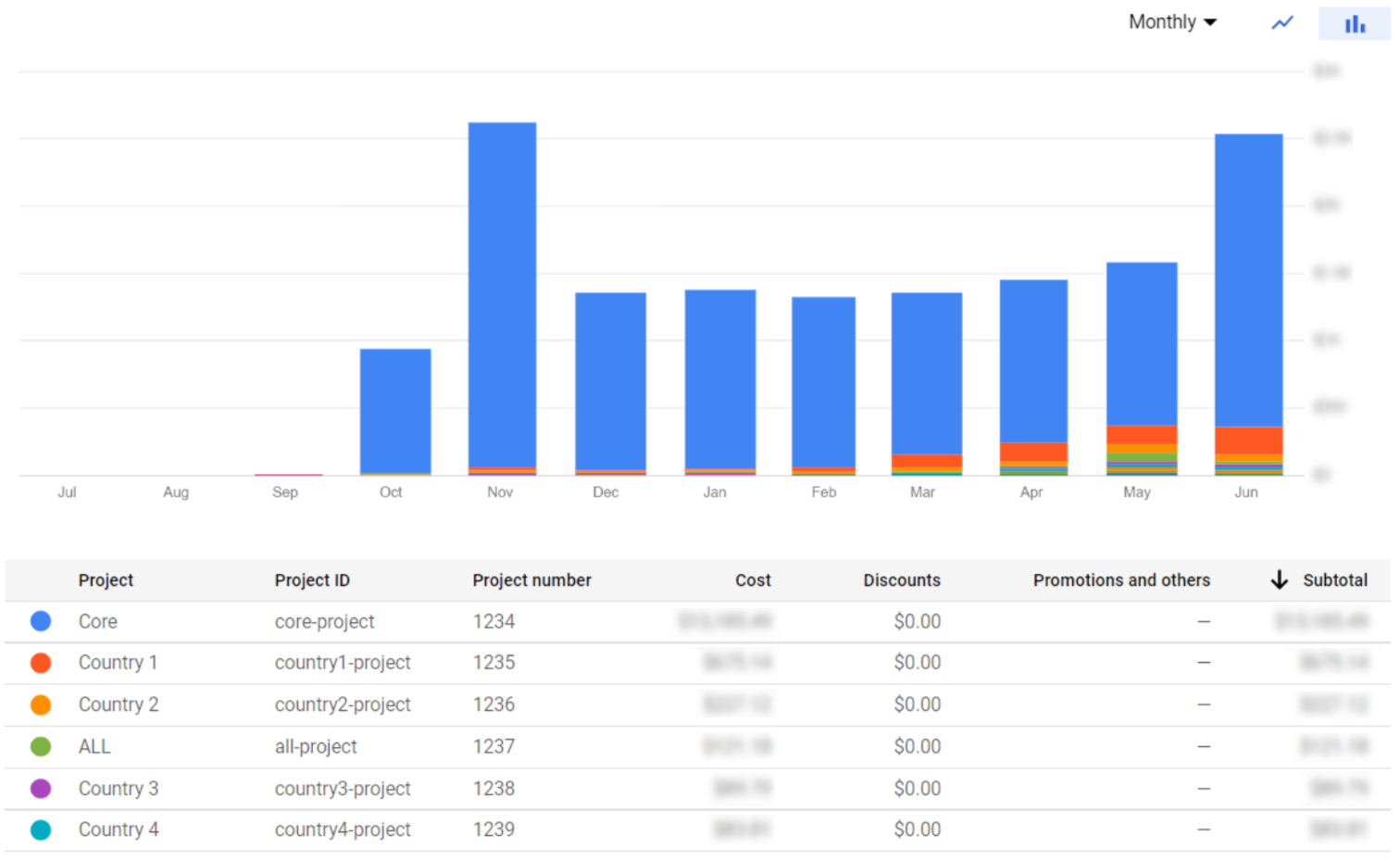
Figure 2: Organisation monthly cost per project

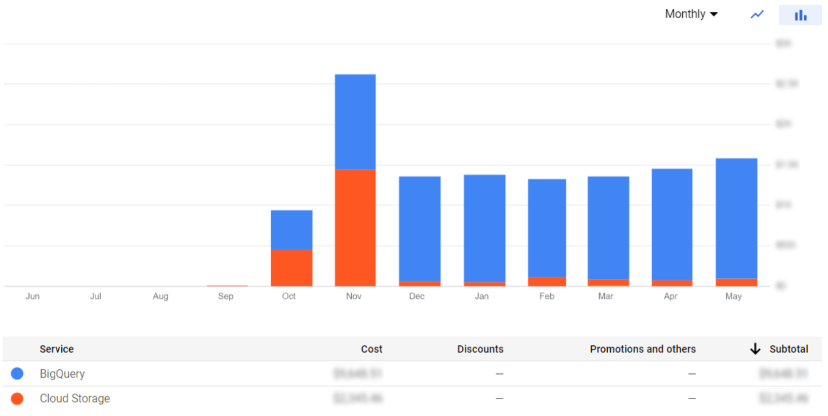
Figure 3: Organisation monthly cost per service

These visualisations are great to give us a clear idea of service and project costs. Nevertheless, we might need a more detailed analysis. In the following sections, we’ll explain how to obtain a complete cost breakdown on both BigQuery and Cloud Storage services.

2. Cloud Storage Cost Breakdown

Cloud Storage is the GCP data lake and object storage service, providing unlimited storage for storing data (objects) in buckets, interoperability with other clouds, strong consistency in its read and write operations, high availability, and access control with ACLs and IAM.

If you remember, in our previous blog post we were storing files both in Standard and Archive classes; the Standard mode is costly to store but cheap to operate, whereas the Archive mode is the opposite – cheap storage and expensive operations. We recommend you take a look at their documentation on Cloud Storage pricing, as understanding the storage classes is really important.

At this point, you may be wondering how much you are being billed for each storage class. This information is useful not only to monitor the cost, but also to see at a glance if the chosen class is the best for your project. To obtain this level of cost breakdown, in the Reports page, set Group by SKU and in Services select only Google Storage. Cloud SKUs (Stock Keeping Units) are the different variations of the product or service.

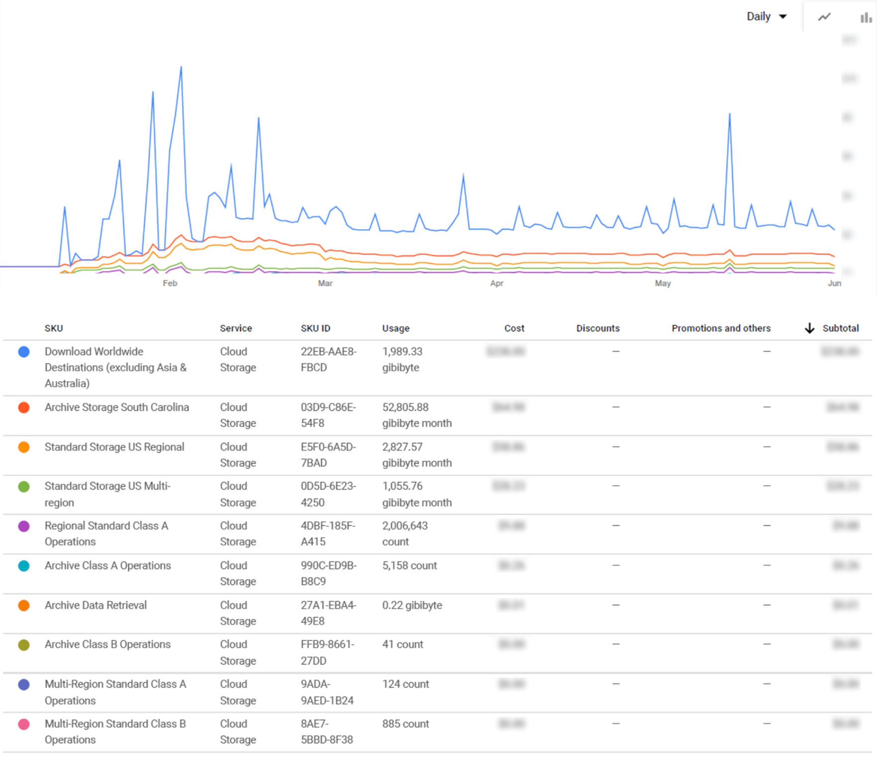
Figure 4: Cloud Storage monthly cost per SKU

Taking a look at the example above (Figure 4), we can see that we have been billed for several different SKUs in one or multiple regions: downloading content, Standard and Archive storage, and Class A and B Operations. In order to better understand the variety of Cloud Storage SKUs, we have prepared below a table that explains all of them and the categories they belong to.

Cloud Storage pricing is divided into four main components:

• Data storage: the amount of data stored in buckets.
• Network usage: the amount of data read or moved.
• Operations usage: operations like adding objects, listing buckets, and so on.
• Retrieval and early deletion fees: additional costs for not complying with the non-standard storage type conditions.

Each is composed of many SKUs, which have been categorised and defined in this table:

Table 1: Cloud Storage SKUs

This table groups together all possible SKUs related to Cloud Storage. Nonetheless, you can find the detailed pricing of Cloud Storage on the pricing page, and the cost of each SKU on Google’s SKUs page.

In the next part we are going to give you an overview of BigQuery cost management, one of the key services not only in our projects but also in the entire Google Cloud Platform.

3. BigQuery Cost Breakdown

BigQuery is the GCP data warehouse and serverless analytics platform, which contains a query engine that processes data in a fast and flexible way. Due to its highly scalable serverless computing model, it automatically allocates the resources on demand, distributing them over several machines working in parallel.

BigQuery pricing is divided into:

• Analysis pricing: the cost of processing different types of queries, such as SQL queries, scripts, user-defined functions, data manipulation language (DML) and data definition language (DDL) statements.
• Storage pricing: the cost of storing data that is loaded into BigQuery, based on the size of the stored data. There are two options available, depending on when the last time the data in the tables was edited. There is no difference between them in terms of performance, durability, or availability.

Each model is composed of two specific SKUs, explained in the following table:

Table 2: BigQuery SKUs

In addition to these, there are other operations that are charged for in BigQuery, such as streaming inserts and reads, and using the BigQuery Storage API. It also offers some free operations, including copying and exporting data, metadata operations, and a free usage tier up to a specific usage limit.

As each project created in GCP is associated with a billing account, all the BigQuery jobs and storage charges that are within the scope of that project will be billed to that account.

BigQuery cost breakdowns can also be found on the Billing Reports page. As with Cloud Storage, we can filter by Service (BigQuery) and its SKUs, to retrieve the total cost per SKU.

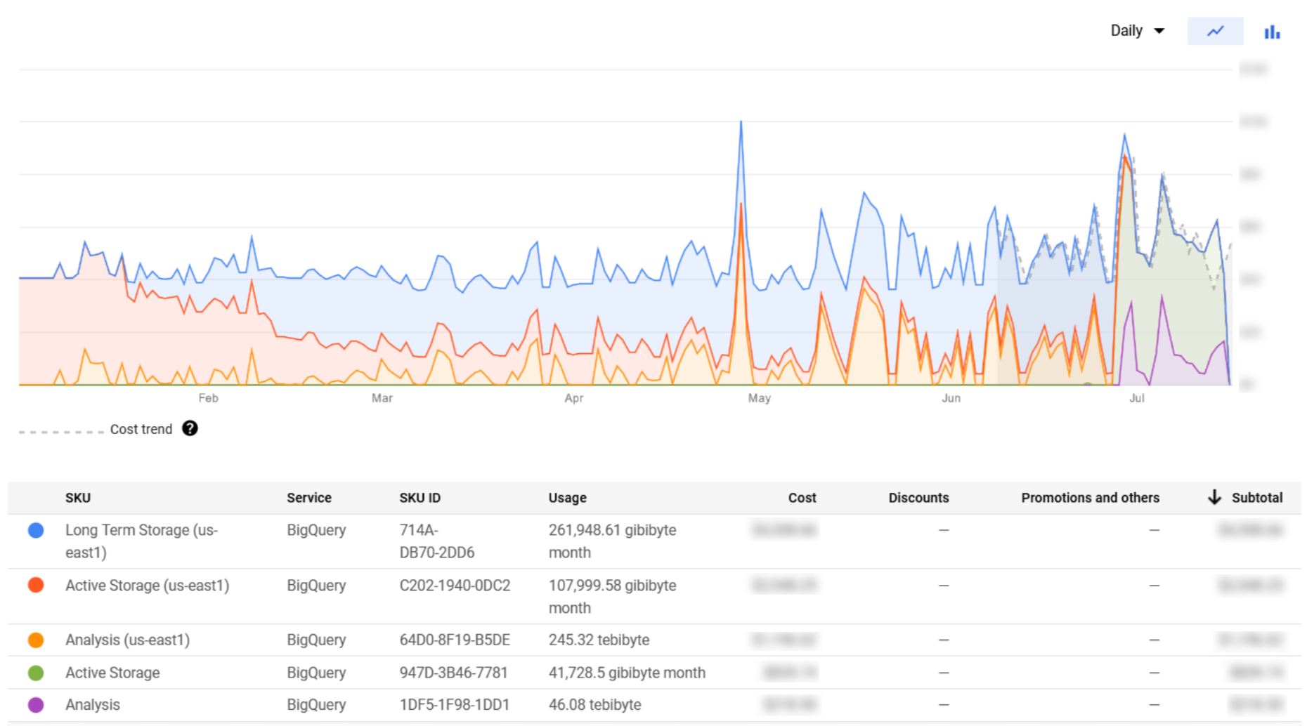
Figure 5: BigQuery monthly cost per SKU

We can observe that the SKUs shown in Figure 5 are more intuitive than the ones retrieved for Cloud Storage. Bear in mind that the BigQuery Analysis cost is directly impacted by the queries performed by users, which can be risky if left unsupervised.

An important mechanism to limit the cost per query and per user are quotas, which were already explained in our first GCP blog post. However, specifically for BigQuery, there is another powerful utility to monitor this service in a more advanced way called information schema.

3.1. BigQuery Information Schema

The information schema provides access to certain metadata tables inside BigQuery that help us to access query history in an SQL-like fashion, obtaining additional information that is not available from the Billing portal.

In this part we are going to list a few interesting insights that can be obtained from querying the information schema tables, as well as some example SQL statements and their results.

Before diving into these examples, we would like to clarify a few concepts. First, the term “job” refers to any action run in BigQuery, such as loading, exporting, querying, or copying data. In this section, we will focus mainly on querying jobs. Furthermore, these jobs have different access levels: there are jobs by organisation, by folder, by project, and by user.

In order to get this type of information by querying the information schema table, you might need some extra permissions like the BigQuery Resource role configured in the IAM service. Note that only jobs from the last six months can be recovered from the information schema metadata.

Below we can see some examples that can be executed from the BigQuery console:

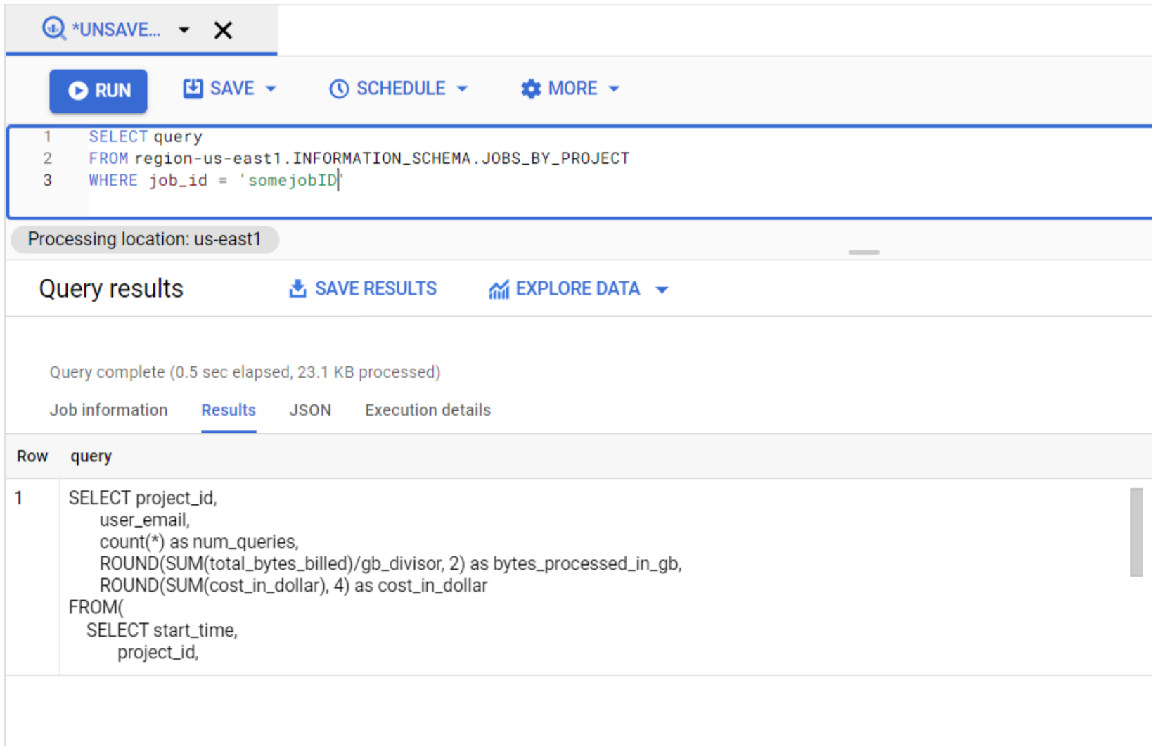
• Retrieve query executed in a specific job: Useful to understand exactly what has been executed, for example, when we notice a peak in the price of a query. Note that you can only get the queries that were executed at a project level (JOBS_BY_PROJECT):

  SELECT query  
  FROM region-us-east1.INFORMATION_SCHEMA.JOBS_BY_PROJECT  
  WHERE job_id = 'job-id'; 
  

   

  

  Figure 6: Information schema query 1

   

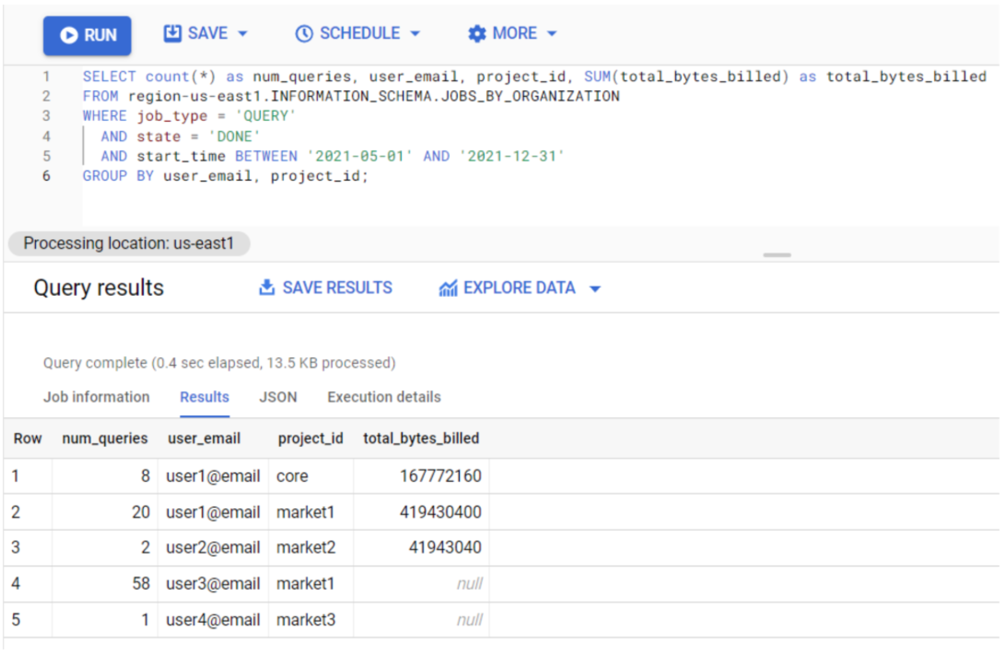
• Count number of queries executed by user and project: With this metric we can get a clearer picture of which users are using the service the most and the least. The result of the query below gives the total number of executed queries and the sum of the total amount of bytes billed per user and project:

  SELECT count(*) as num_queries, user_email, project_id, SUM(total_bytes_billed) 
  as total_bytes_billed
  FROM region-us-east1.INFORMATION_SCHEMA.JOBS_BY_ORGANIZATION 
  WHERE job_type = 'QUERY'  
    AND state = 'DONE' 
    AND start_time BETWEEN '2021-01-01' AND '2021-05-31' 
  GROUP BY user_email, project_id; 
  

   

  

  Figure 7: Information schema query 2

   

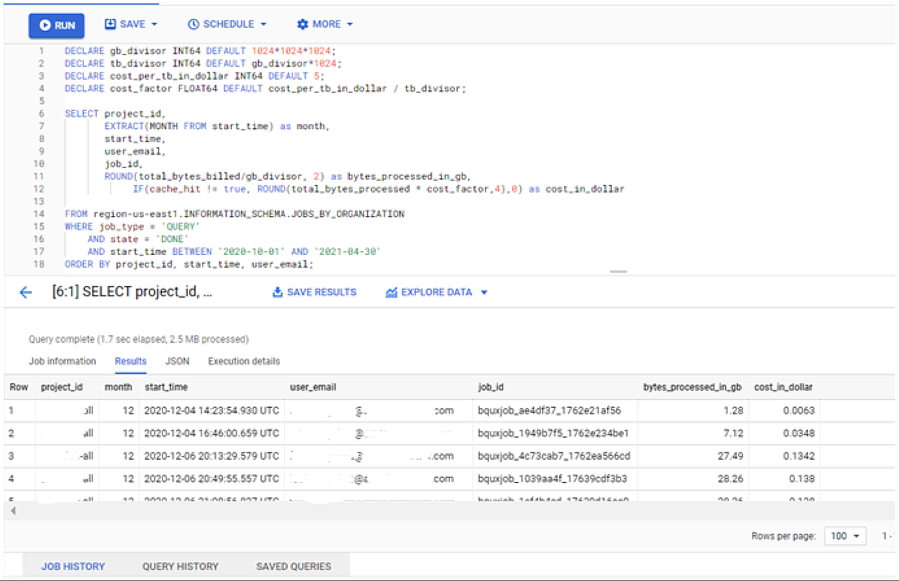
• Query history by user and project: In addition to this historical information, it provides an estimation of the cost for each query:

  DECLARE gb_divisor INT64 DEFAULT 1024*1024*1024;  
  DECLARE tb_divisor INT64 DEFAULT gb_divisor*1024;  
  DECLARE cost_per_tb_in_dollar INT64 DEFAULT 5;  
  DECLARE cost_factor FLOAT64 DEFAULT cost_per_tb_in_dollar / tb_divisor;      
  
  SELECT project_id,   
         EXTRACT(MONTH FROM start_time) as month,   
         start_time,   
         user_email,   
         job_id,   
         ROUND(total_bytes_billed/gb_divisor, 2) as bytes_processed_in_gb,  
         IF(cache_hit != true, ROUND(total_bytes_processed * cost_factor,4),0)
         as cost_in_dollar  
  FROM region-us-east1.INFORMATION_SCHEMA.JOBS_BY_ORGANIZATION  
  WHERE job_type = 'QUERY'   
      AND state = 'DONE'  
      AND start_time BETWEEN '2020-10-01' AND '2021-04-30'  
  ORDER BY project_id, start_time, user_email; 
  

   

  

  Figure 8: Information schema query 3

   

The output of the queries can be seen in a tabular format in the same portal after execution, or downloaded in different file formats such as CSV. However, we recommend you create your own personalised dashboards using the results of these queries as sources in Data Studio to monitor the usage of your queries in a more visual way.

As we commented above, BigQuery has two pricing models: on-demand and flat-rate. If you are using a combination of both, you might also want to include the column “reservation_id” in your INFORMATION_SCHEMA queries to distinguish queries executed in flat-rate or on-demand pricing models. When a query is executed in flat-rate (and this is done by purchasing Reservations), the “reservation_id” will have a non-NULL value, while the “reservation_id” will be NULL if the query was executed in the on-demand pricing model.

In addition to the queries that we have introduced here, there are many others that can help you to monitor BigQuery costs in more depth. To find out more about this, take a look at their official documentation.

Conclusion

Monitoring cloud service costs might seem challenging, but as we have seen in this article there are some useful monitoring tools, focusing on Cloud Storage and BigQuery, to help you to achieve this task by understanding the details of the provider’s billing page and the information schema for BigQuery.

If you are planning on creating a data platform or if you are having a hard time trying to understand your billing, please do contact us as we have a lot of experience in building cost-effective cloud infrastructures and defining secure quotas that fulfil your business requirements.