
29 Nov 2021 Data Lake Querying in AWS – Athena
This article is the second in the ‘Data Lake Querying in AWS’ blog series, in which we are introducing different technologies to query data lakes in AWS, i.e. in S3. In the first article of this series, we discussed how to optimise data lakes by using proper file formats (Apache Parquet) and other optimisation mechanisms (partitioning), and we introduced the concept of the data lakehouse.
We also presented an example of how to convert raw data (most data landing in data lakes is in a raw format such as CSV) into partitioned Parquet files with Athena and Glue in AWS. In that example, we used a dataset from the popular TPC-H benchmark; essentially, we generated three versions of the TPC-H dataset:
- Raw (CSV): 100 GB; the largest tables are lineitem with 76GB and orders with 16GB, and they are split in 80 files.
- Parquets without partitions: 31.5 GB; the largest tables are lineitem with 21GB and orders with 4.5GB, and they are also split into 80 files.
- Partitioned Parquets: 32.5 GB; the largest tables, which are partitioned, are lineitem with 21.5GB and orders with 5GB, with one partition per day; each partition has one file and there are around 2,000 partitions for each table. The rest of the tables are left unpartitioned.
In this blog post and the next ones, we will be presenting different technologies that can be used for querying data in a data lake, so we can consider them as building blocks for a data lakehouse. We will be using, as a common dataset, the three versions we generated in our first blog as seen above; so make sure you have read that blog post before proceeding with this one! Each of the technologies we present has its pros and cons, and choosing which is the best for you depends on many variables and requires a thorough analysis. We would be happy to help you with such an analysis so do not hesitate to contact us.
Please bear in mind that these blogs only aim to present various technologies and to show you how to use them; in all the blogs we start with the three versions of the TPC-H dataset sitting in S3 and we will describe how to load them (if they require loading) and how to query them.
The queries that we will use are those offered in the TPC-H specification document. Specifically, we will execute queries 1, 2, 3, 4, 6, 9, 10, 12, 14 and 15. Some of the characteristics can be seen in the following table:
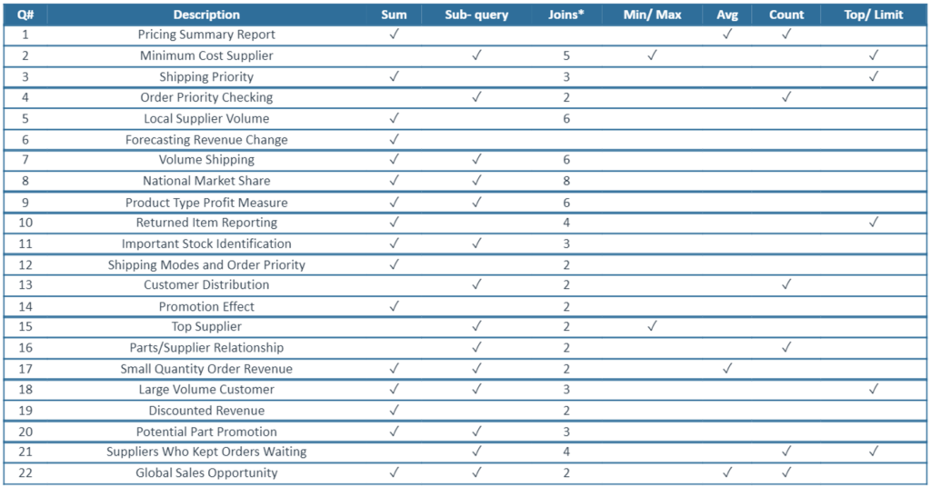
Source: Actian
Most of these queries make use of filters by date, generally the column l_shipdate from the lineitem table and the column o_orderadate from the orders table. These fields are the ones by which we partitioned both tables in the version of the dataset where we partitioned the two largest tables.
Moreover, we are also going to discuss how the various technologies can connect to reporting tools such as Tableau.
So now let’s focus on our first option – in this blog post, we are going to explain how to use Athena to query the 3 different versions of the TPC-H dataset, as well as how to connect Tableau to Athena.
Introducing Athena
Athena is an important serverless service of AWS – key for the data analysts, engineers and scientists using AWS. It is an intuitive and easy-to-use query service with no administration required, and you only pay for the data scanned in the queries you make. Leveraging data compression or using columnar formats might reduce scanned data, and thus cut costs.
Athena is simple to configure: it only needs a data storage such as S3 and a Data Catalog.
In addition to these costs, the external services used are also billed. As Athena is serverless, it needs extra services to contain and structure the data. And remember that DDL operations (such as CREATE, ALTER and DROP), partition administration, and failed queries are free of charge.
It is also important to know how it works: Athena is a combination of Presto syntax and ANSI SQL.
Athena has several limitations that are worth noting: there are 600-minute timeouts on DDL operations and 30-minute timeouts on DML; there are also limitations on data structures, with a limit of 100 databases, 100 tables per database and 20,000 partitions per table. Scalability might be an issue for large projects, as you need to contact AWS to increase capabilities.
Now that the presentations are over, let’s get down to it!
Hands-on Athena
One of the characteristics of Athena is the easy-to-use interface: queries can be executed in its own query editor, but there is a limitation of 10 tabs open simultaneously.
Creating the Schema Definitions
Before starting to query, the data must be prepared.
Note that Athena itself is just a querying engine on top of S3, not a data store, and it leverages Glue Data Catalog to store the definition of databases and tables. We will need to create a database and table schema definitions which will be stored in the catalog. These schema definitions can be checked using AWS Glue. Note also that Athena stores related metadata and results in S3.
Let’s start with the first version of the dataset, the raw (CSV) one. The first thing to create is a database:
CREATE database IF NOT EXISTS tpc_db;
Then tables can be created with the following code (example for the table orders):
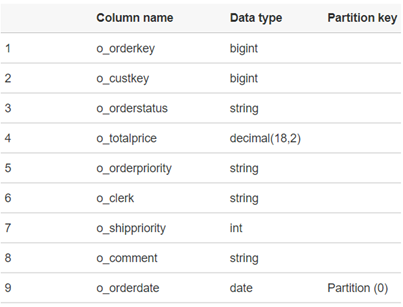
CREATE external TABLE tpc_db.orders(
    o_orderkey BIGINT,
    o_custkey BIGINT,
    o_orderstatus varchar(1),
    o_totalprice float,
    o_orderdate date,
    o_orderpriority varchar(15),
    o_clerk varchar(15),
    o_shippriority int,
    o_comment varchar(79)
)
ROW FORMAT DELIMITED
FIELDS TERMINATED BY '|'
STORED AS textfile
LOCATION 's3://athena-evaluation/tpc-h-100gb/orders/';
Note that the keyword ‘external’ is used to specify that this table is not stored internally. This is because Athena doesn’t manage the data or its metadata; everything is handled by AWS Glue.
Moving on to our next version of the dataset, the unpartitioned Parquets, the syntax to create the database and one of the external tables (orders) would be:
CREATE database IF NOT EXISTS tpc_db_par;
CREATE external TABLE tpc_db_par.orders(
    o_orderkey BIGINT,
    o_custkey BIGINT,
    o_orderstatus varchar(1),
    o_totalprice float,
    o_orderdate date,
    o_orderpriority varchar(15),
    o_clerk varchar(15),
    o_shippriority int,
    o_comment varchar(79)
)
STORED AS Parquet
LOCATION 's3://athena-evaluation/tpc-h-100gb-par/orders/';
Finally, for the last version of the dataset, the partitioned Parquets (only the largest tables are partitioned), the syntax to create the database and one of the external tables (orders) would be:
CREATE database IF NOT EXISTS tpc_db_opt;
CREATE external TABLE  tpc_db_opt.orders(
    o_orderkey BIGINT,
    o_custkey BIGINT,
    o_orderstatus varchar(1),
    o_totalprice float,
    o_orderdate date,
    o_orderpriority varchar(15),
    o_clerk varchar(15),
    o_shippriority int,
    o_comment varchar(79)
)
PARTITIONED BY (o_orderdate date)
STORED AS Parquet
LOCATION 's3://athena-evaluation/tpc-h-100gb-opt/orders-part/';
If there is a partition in the data, the command MSCK REPAIR table_name must be executed to load the necessary metadata and enable the correct usage of the table that contains the partitioned data.
As mentioned above, to verify that everything has gone well, you can go to AWS Glue and check that the database that has been created:
Running the Queries
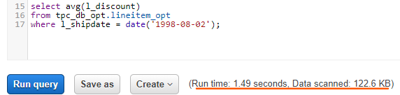
Once everything has been set up, queries can be executed. As mentioned above, we ran 10 queries from the TPC-H specification for each version of the dataset. Note that when running a query, the query execution time as well as the data scanned are shown below the writing box:
There is also a history tab on the upper side of the window, where previous executions can be seen. If you click on one of the queries, it is shown in the query editor so that the original code may be recovered.
When comparing the results of running the queries in the three different versions of the dataset, we have observed that the use of Parquet is highly beneficial, not only because it reduces the cost, but also because it is faster to read. On average, we have observed an improvement factor of 2-3x when using Parquet compared to CSV. It makes sense, since the Parquet format is columnar, which improves performance in analysis queries such as those that the BI team would make, and it is also smaller as it is binary and compressed.
Regarding partitioning, though query times decrease in general, there is not much difference in the execution time compared with the unpartitioned Parquet, because the dataset we used was not large enough. With a bigger dataset, an improvement in time would be noticeable. Although not that different, the amount of data scanned is slightly lower with partitioning, and that means less cost.
Note that each query uses independent compute resources, so with high user concurrency there are no mechanisms to optimise compute resources, and costs can go up very quickly.
Tableau Connection
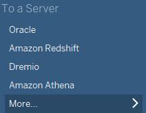
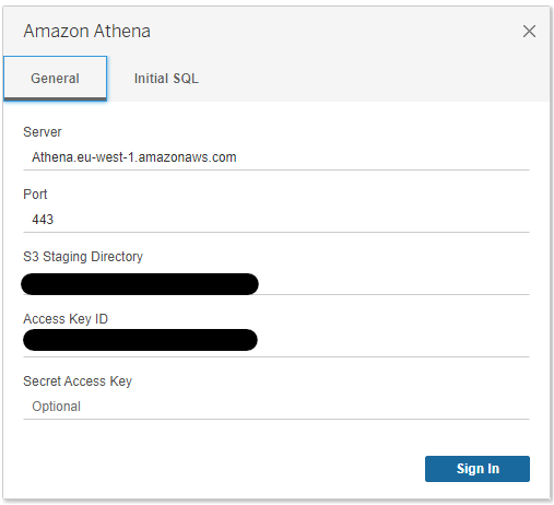
The connection between Athena and Tableau is simple to make: there is an option to use Athena as a data source, though you need to install a driver to connect to Athena first.
Setting up the connection requires the endpoint of the server you are connecting to, depending on the region. The server’s name per region can be found in the Amazon Athena endpoints and quotas reference guide in the AWS documentation.
It also requires an S3 directory which will be used as a staging directory to save data and metadata related to the queries executed in Athena. As identifying credentials, access keys are used. To learn more about access keys, read the Managing access keys for IAM users user guide in the AWS documentation. After you sign in, use Tableau as usual:
Note that Tableau does not perform well with JOINs when large tables are involved, so in some cases it is advisable to have these JOINs precomputed at the database / data lake level before using the dataset for reporting purposes to avoid time-consuming queries.
Additionally, it may help to create aggregated tables depending on the use case. Furthermore, Tableau has its own query planning, and this might present a certain risk with Athena, because the user might not control the amount of data scanned and this could lead to an unexpectedly high cost. So, when using Athena with Tableau, you really must know what you are doing, and you must have structured the underlying data very well.
Athena – Pros and Cons
In this article we have presented Athena, and the advantages that we would like to highlight are:
- It is a serverless query service which is very easy to start with and does not require you to set anything up.
- It allows querying directly to S3 without an infrastructure.
- Preparing Athena for querying data in S3 is as easy as running a few DDL statements to define schemas in a catalogue.
- Its pricing is pay-per-query and it is very simple to monitor costs.
- It is an excellent choice for relatively simple in-lake (S3) ad hoc queries, and if the S3 data lake is properly organized, we get very good performance. We have tested running the same queries with the three different versions of the same dataset and we have seen the impact (factor 2-3 improvement) of using an optimised file format such as Parquet. We have also seen a small gain when using partitioning (our dataset was too small to see a significant gain).
- It is fully compatible with AWS Glue.
However, while we believe Athena is great, there are few things to consider:
- The drawback of being serverless and fully managed is that there are very few options in the administration and tuning of the engine itself. Tuning Athena is not immediate, you need to contact AWS to increase its capabilities.
- Athena is designed for running relatively simple queries, and users must know what they are doing, especially when dealing with reporting tools, or there could be unexpected costs.
- Since each query is independent, when dealing with many users or highly concurrent scenarios, the engine itself and, more importantly, its cost, cannot really leverage the concurrency to optimise itself.
Conclusion
Athena is a good choice for querying data in AWS lakes, but in some cases it may not be the best. In some situations, such as when complex queries are involved, or there is an extensive use of BI tools, or high concurrency, one needs to think very carefully about how to select the best approach.
One approach is to optimise the data lake tables further by creating joined or aggregated tables; another approach is to use a data warehousing technology such as Redshift, which is exactly what we will cover in our next blog post. Redshift also allows querying directly in S3 with Spectrum, as well as loading data to the warehouse – thus increasing performance on complex queries and avoiding being charged for data scanned (though Spectrum does charge per data scanned in S3).
Actually, what AWS proposes as a lakehouse is the combination of S3, Athena, and Redshift. If you are interested in the differences between Athena and Redshift and when to choose one over the other, we recommend this blog article. There are also other approaches, which we will be covering in the upcoming blog posts in this series.
If you are interested in using Athena or any other AWS service, or are wondering what the most suitable architecture for your data platform is, simply contact us. Here at ClearPeaks we have a broad experience with cloud technologies, and we can help you decide on the best option for your projects.
The blog series continues here.