29 Dec 2021 Data Lake Querying in AWS – Dremio

This is the sixth and final article in the ‘Data Lake Querying in AWS’ blog series and it’s been a long ride, so thanks for staying with us! In this series we have introduced different technologies to query data lakes in AWS, i.e. in S3. In the first article, we discussed how to optimise data lakes by using proper file formats (Apache Parquet) and other optimisation mechanisms (partitioning); we also introduced the concept of the data lakehouse. We demonstrated a couple of ways to convert raw datasets, which usually come in CSV, into partitioned Parquet files with Athena and Glue, using a dataset from the popular TPC-H benchmark from which we generated three versions:

• Raw (CSV): 100 GB, the largest tables are lineitem with 76GB and orders with 16GB, split into 80 files.
• Parquets without partitions: 31.5 GB, the largest tables are lineitem with 21GB and orders with 4.5GB, also split into 80 files.
• Partitioned Parquets: 32.5 GB, the largest tables, which are partitioned, are lineitem with 21.5GB and orders with 5GB, with one partition per day; each partition has one file and there around 2,000 partitions for each table. The rest of the tables are left unpartitioned.

We have presented various technologies to query data in S3: in the second article we ran queries (also defined by the TPC-H benchmark) with Athena and we compared the performance  depending on the dataset characteristics. As expected, the best performance was observed with Parquet files.

However, we determined that for some situations a pure data lake querying engine like Athena may not be the best choice, so in the third article we introduced Redshift as an alternative for situations in which Athena is not recommendable. As we commented in that blog post, Amazon Redshift is a highly scalable AWS data warehouse with its own data structure that optimises queries, and in combination with S3 and Athena, can be used to build a data lakehouse in AWS. Nonetheless, there are many data warehouses and data lakehouses in the market with their own pros and cons, and depending on your requirements there may be other more suitable technologies.

In the fourth article we introduced Snowflake, an excellent data warehouse that can save costs and optimise the resources assigned to our workloads, going beyond data warehousing as it also tackles data lakehouse scenarios in which the data lake and the transformation engine are provided by the same technology.

Following the data lakehouse discussion, in the fifth and latest article, we talked about Databricks and its lakehouse approach, the idea of which is also to keep the workloads in a single platform but without duplicating or importing any data at all, so all data can stay in S3. Following on from this idea of decreasing imports and duplications, we explained that as an alternative there is a technology called Dremio, which is a data lake querying engine whose paradigm differs from the rest of the technologies we have seen in this series.

In this article, we will look at the basics of Dremio and see how we can leverage our data lake without duplicating any data. Then, we will go through a hands-on example to see how Dremio is used, how to use it with Tableau and, finally, we will conclude with an overview of everything Dremio has to offer.

Introducing Dremio

Dremio is a cloud-based data lake engine whose main objective is to offer the ability to deal with a large amount of data on an end-user level (BI, analytics…) directly from data lakes with simultaneous multiple sources.

The wide compatibility that Dremio offers can help to simplify the workflow of a project, although it does not cover every stage of the data lifetime; for example, to apply transformations to the data you will still need to use other services.

There is a SaaS alternative in development called Dremio Cloud. The goal of this project is to ease access to data even more and remove the necessity of having to access physical machines while maintaining high scalability. At the time of writing, Dremio Cloud is still in development and there is not yet any publicly available version. Currently, Dremio  must be deployed in a physical machine for which you pay for every second that it is running. In this article, Dremio is used on AWS, so the instances for which you pay are EC2.

If you are using the Dremio Enterprise edition, you also have to pay for the license, the price of which scales along with the EC2 instance price. Check Dremio’s pricing in the AWS Marketplace for more detailed information; using the marketplace also eases deployment efforts.

The way Dremio improves performance is by using virtual tables which can contain precalculated values, sorting, partitioning, etc. Because of this, Dremio relies heavily on external storage to store these modified virtualisations, called reflections.

Please note that Dremio uses temporal (EC2) instances called Elastic Engines for which the user must pay as well.

The Elastic Engine concept might be better understood after looking at the Dremio architecture.

Dremio Architecture

Dremio follows a leader-worker architecture: the leader or coordinator node is the first created during the initial deployment, and the workers are called Elastic Engines, which are temporary EC2 instances that are used for most queries. These Elastic Engines are easily deployable and can be customised like other EC2 instances.

The administration of these engines also allows you to separate the execution by queues, so that one node can be dedicated to computing high-cost queries while the others take care of everything else. You can also limit the number of nodes that can be created.

There is another key concept that must be understood to get the most out of Dremio: a reflection.

Reflections

Dremio offers the possibility of keeping physically optimised sets of data from the source; these optimisations are called reflections. When a query is executed, Dremio selects reflections which accelerate it instead of processing the data. A query accelerated by an existing reflection means that this reflection covers the query.

Using a reflection does not mean that the query is being completely covered (although this might happen); it is common to partially cover it as it is a more realistic use case. If multiple reflections cover a query, the best one is automatically chosen. To understand what we mean by “cover”, imagine a query with a subquery; maybe the subquery fits completely with a reflection, but the query itself does not. So, in this case we can say that the query is partially covered by a reflection.

There are two main types of reflection: raw and aggregate.

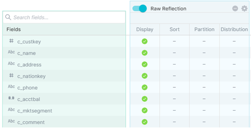
Raw reflections are always advisable when a plain text format is in the data source, so that formats like CSV or JSON are faster to query. Among the options of reflections per column there are:

• Display (typically done for all used fields)
• Sort
• Partition

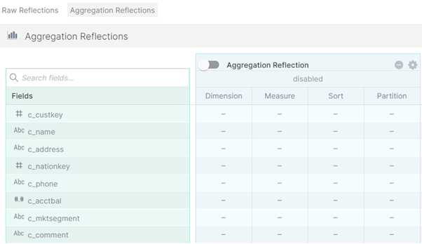
On the other hand, aggregation reflections are used to accelerate queries for analytical purposes, like BI. The options to reflect offered for each column are:

• Dimension: for columns that appear in GROUP BY, DISTINCT or in filters like WHERE column1 IN (…)
• Measure (sum, count, max, min, approx. distinct count)

• Sort
• Partition

We will not dive deeper into reflection use cases in this article, but we highly recommend taking a look at the official documentation about reflections; reflections are not difficult to understand – in fact, thanks to the naming selected by Dremio, they are intuitive.

Reflections are stored outside the instance running Dremio, and rely on the  data lake used as the data source. In this case, as we are using S3 as the data lake, all reflections will be stored there as well. Having to work with external data may slow down executions, and the creation of reflections may take more time than most queries; to maintain lower times, create reflections over compressed data. Moreover, it is interesting to bear in mind that other reflections can be used for the creation of new ones.

This might sound great, but how much effort is required to handle reflections?

Good news – almost none!

Dremio offers an option to automatically update reflections. This is very useful indeed to avoid administrative costs with the arrival of new data to the data source. These updates can also be deactivated if no more data is expected or if you want to do it manually.

The updates are done as a broadcast, starting from the root, which is the data source, and the changes are propagated to the virtualisations generated on top of the previous data. The old version of a reflection remains available until the update is finished, then a job to remove the old version is queued.

Besides the refresh time there is also an expiration time, after which the reflection will be invalidated; only if there is a new version of the reflection will it still be available. With the expiration time, we ensure that the reflections that are no longer used are removed.

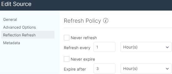
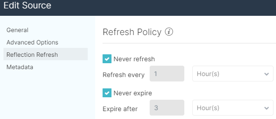
The rules for updating reflections can be general or specific for each data source:

Reflections that take a long time to be created might be a problem if their duration is not considered and the refresh time is not modified appropriately.

For example, in the case of a reflection that takes one hour to be created and whose update is scheduled every hour as well, during the refresh time the previous reflection will be used, and when the creation finishes this new one will be used, but there will always be a job running in the background, which could lead to reduced performance. It could get even worse if the creation of a reflection lasts more than the specified refresh or expiration time.

The removal of expired reflections is not instant either; a job is executed in the background, but contrary to updated reflections, the expired reflections stop being available when the timer triggers, even if they have not yet been removed.
Note that when Dremio removes its data from S3, objects are removed but the folders remain visible, so it is possible that at some point the Dremio S3 bucket is filled with empty folders.

With all these issues associated with the renewal of data, let’s look at what we can do to avoid them.

The risk of slow queries may increase depending on the amount of memory needed to finish them, so it is important to consider the resources available to avoid lower performance.

If an entire query cannot be handled in memory, there are cases in which the disk might be used to finish them, called “spilling a query” in Dremio. The disk is mostly used for aggregations; in the case of joins, spilling is not used.

For most queries, the use of reflections will reduce the amount of memory needed to compute them. Even so, spilling can be used in the creation of reflections as well. In this case, it might be decreased by making incremental virtualisations; general virtualisations should be created first and then more precise ones can be built on top of them, and then finally, reflections should be created on the most accurate queries.

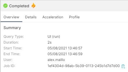
The memory consumption of the executed queries can be monitored from the Dremio job history, in the Profile tab:

Scrolling down in the Overview tab, you will find some general metrics related to memory consumption:

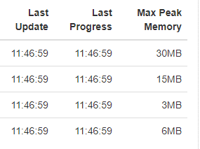
There is plenty of information related to executed queries in this Job Profile window, and it is very useful to check and monitor how queries are doing.

After this technical dive, let’s focus now on getting started with Dremio.

The deployment of Dremio in AWS is done from the marketplace and can be launched in CloudFormation. There is an official step-by-step video guide to deployment in AWS.

There is also a Docker image with which you can try it locally for free before getting into advanced projects.

After deploying Dremio in our AWS environment, we can start to query data from the TPC-H dataset in S3 in its multiple versions.

Hands-on Dremio

To connect Dremio to the data source, there is a button in the lower left corner in the UI where you can add a data lake. In the window that appears, we select S3 and enter the AWS credentials to connect. In the Reflection Refresh tab, we check the boxes “Never refresh” and “Never expire”, as we will not have new data for this hands-on example.

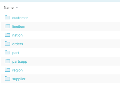
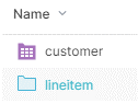
Now we must specify which S3 resources we are going to use: the objects we select will be the physical layer and we will only specify what format they have – they will not be loaded or moved anywhere. To add a new object as a physical table, go to the data lake and search for the desired object:

Then click on the transformation button that appears when hovering the mouse over an object:

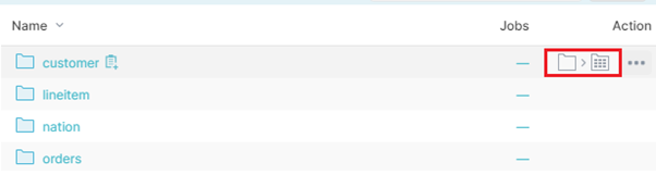
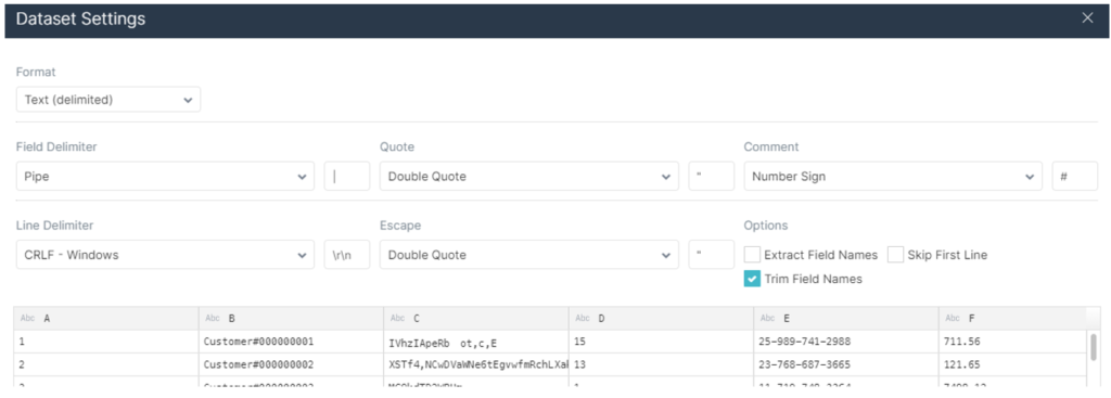
A new window pops up. If the right format is not automatically detected, specify it:

After saving the changes the object will be seen as a folder icon with a grid, meaning it is a physical dataset:

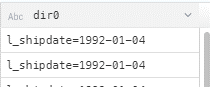
It is straightforward to specify the format in which the data is held in the data lake. However, the reading of partitioned data is not directly detected if it is in a Hive format; Dremio detects folders named ‘dir0=value’:

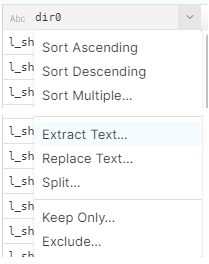
To change that, go to the target field and select the ‘Extract text’ option, in the dropdown menu:

Then select how you want to extract the text. We selected by position:

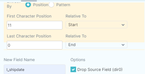
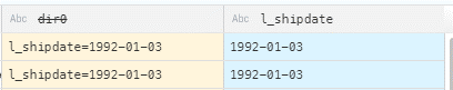
Make sure you mark the checkbox to drop the source field. The result will be displayed as a preview before applying the changes, and should look like this:

This can be saved as a virtualisation as the physical dataset cannot be changed.

Let’s take another step forward and start with the creation of reflections.

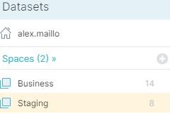
First, we will create a first virtualisation layer which we will call the Staging layer. We go back to the main menu, and folders can be created to maintain everything in good order. This layer will be represented by a new folder:

For this layer we will virtualise all tables using one-to-one virtualisation. To create a virtualisation, go to one of the physical sources and click on it to open the preview and the SQL text field. Change the names and the types of the fields if necessary, and click on ‘Save as’ and save it in this first Staging folder.

Virtualisations are shown as a square icon filled with a grid.

Now that the virtualisations have been created, we can create reflections from them to accelerate queries. To create reflections, click on the settings button that appears when hovering the mouse over a virtual table, and select the reflections tab in the window that appears.

The first thing shown here is the basic menu; some fields are automatically recommended to put in both raw and aggregation reflections. However, we recommend going to the Advanced view:

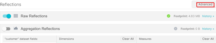
In the Advanced view there are more properties to give to each field, and it can further reduce execution time.

Also note that it is possible to have multiple reflections for the same virtualisation, which can help prepare a general business layer to then create multiple analytical and more precise reflections without having to create a virtual table with the same data for every use case.

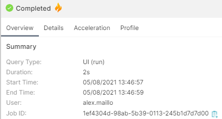
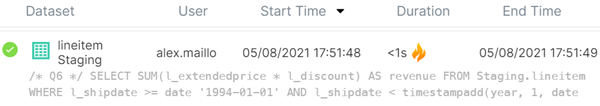
Once all the reflections have been created, we can start executing the queries. To check if they are being accelerated you can look at the Jobs tab, where all the executed queries are stored as a history. If a flame icon appears in the Duration column, that means the query has been accelerated:

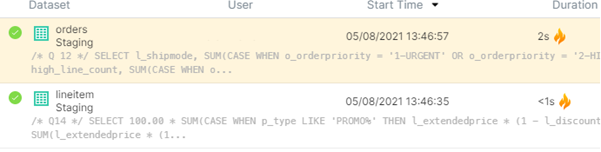
You can look for more information in the tabs on the right side of the page:

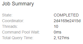
The exact execution time is shown in the Query tab of the query Profile, scrolling down to a section called Job Summary:

Let’s focus now on one of the queries from the TPC-H dataset and try to accelerate it.

If our dataset is in plain text format, like the first version of out TPC-H datasets, we will notice a great improvement just by creating raw reflections of each table with all the fields marked as ‘Display’:

However, if we use the Parquet version of the dataset, we can further reduce our query time.

To make it more specific, we are going to accelerate query 6 of the TPC-H dataset:

/* Q6 */

SELECT
     SUM(l_extendedprice * l_discount) AS revenue
FROM
     Staging.lineitem
WHERE
     l_shipdate >= date '1994-01-01'
     AND l_shipdate < timestampadd(year, 1, date '1994-01-01')
     AND l_discount BETWEEN .06 - 0.01 AND .06 + 0.010001
     AND l_quantity < 24;

This query contains an aggregate on the product of two fields with several fields as filters.

One way to create a reflection would be to do it from the one-to-one virtualisation of ‘lineitem’ in the Staging layer. From there, we can create another virtualisation with the field ‘revenue’ added, so that the field is already calculated and it can be seen as a sum in the aggregate reflection:

This is a more general approach, but we are using the whole table just for some fields.

Another way to do it would be to create a virtualisation as simple as the following:

/* Q6 – virtualization */

SELECT
l_extendedprice * l_discount as revenue, l_shipdate, l_discount, l_quantity
FROM
Staging.lineitem;

In addition to the revenue field, we also select the fields that are filtered in the ‘where’ clause in order to show these fields in the reflection menu. The reflection would look like this:

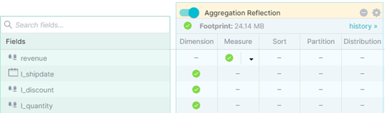
This way we can get smaller and more accurate reflections.

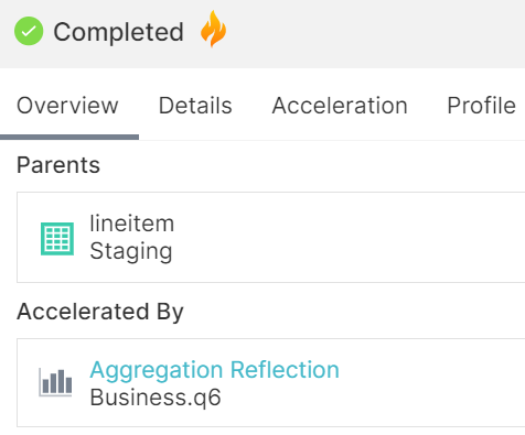
We can run the query and check that it is being accelerated:

On the right side of the Jobs tab, we can also check which reflection is accelerating it:

After executing the queries with CSV, Parquet, with and without reflections, we have noticed that the raw reflections only improve the CSV dataset and do not affect the Parquet positively. Raw reflections should only be used when the dataset is not compressed or in columnar format, or if there are some partitions that have not been made yet.

Regarding aggregate reflections, the execution times of the accelerated queries can be drastically lowered depending on their accuracy, and they also help to avoid the spilling of large queries. Some reflections will take more time to be created when their output size is larger, so before starting with large reflections it is advisable to consider the use of smaller ones to ease the creation of new, bigger reflections.

Tableau Connection

As we have done for the rest of the tools presented in this blog series, we will now discuss how to connect Dremio to a reporting tool such as Tableau. The connection to Dremio is fully supported by Tableau, and there is no need for extra drivers.

From the Dremio UI, for each table, physical or virtual, a file with it already connected and set up can be downloaded; this is a .tds file in the case of Tableau, or a .pbids, if using Power BI.

To get this file we can go to the desired table and click on any of the related BI engine icons in the upper side:

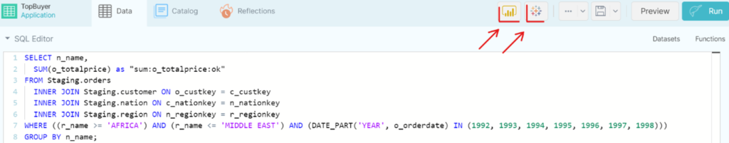
After it has been downloaded, we can simply execute it and it will automatically open Tableau and ask for Dremio credentials. One we have logged in, the selected table will be already prepared for use.

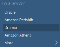
However, there is also the possibility to connect directly to the data source. To do this, Dremio can be found among the data source options:

To establish a connection an IP of the EC2 instance running Dremio must be specified. By default, the port used with Tableau is 31010, as you can see in the image below. A username and password are also needed; these credentials are for Dremio, not for AWS.

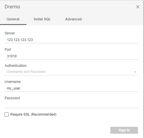
Once signed in, Tableau can be used as usual.

A relevant benefit of Dremio is that you can create specific virtualisations with already precomputed joins and with the corresponding reflections (without duplicating data), allowing the reporting tool to directly query on that virtualisation, leveraging the accelerations and Dremio’s cache system.

Conclusion

Dremio brings high speed to analytical processing without the need of a data warehouse, although it stores reflections in S3. It also simplifies data workflow to ease its usage for different purposes (data scientists, BI, data engineers, etc.). To get the most out of Dremio, it is necessary to learn how it works and to understand reflections, when to use them, and how to avoid bad performance on long reflection creations; its UI makes everything a lot easier.

Dremio brings many benefits as a data lake engine, such as:

• Multiple cloud support.
• Live multi source.
• New data can be automatically refreshed.
• Elastic Engines for better queue distribution and cost effectiveness.
• Good UI with support for more people to work simultaneously.

However, there are some points that should be taken into consideration:

• Partitioned data is supported but it does not detect Hive format partitions.
• Virtualisations and reflections must be properly understood.
• Some reflections might be slow to create.
• Extra nodes are needed to avoid lower performance if reflections change frequently.

Without a doubt, Dremio is a service for data lake querying with a very different approach from the others. It achieves the performance of a large warehouse without the need to load the dataset. As an alternative it presents reflections, which although being physical representations of the data, can be stored directly in the data lake without affecting the execution time.

In this series, we have delved into various data lake querying engines, all of them with their specific strengths. Besides Athena, a simple and powerful querying service in AWS that is extremely useful for ad hoc queries without any configuration, all the other engines follow the lakehouse architecture that we have explained during the series. However, as we have seen, each engine has its own idea of lakehouse architecture.

Redshift is the AWS scalable data warehouse service that, with Spectrum, allows querying data lakes. Traditionally, the architecture has been oriented towards the data warehouse being the central point of data, following an ETL approach. However, the current trend is to follow an ELT architecture, with the data lake as the central data repository. Redshift in concrete is advancing towards that architecture, relegating service as a querying engine and improving querying capabilities with AQUA.

Snowflake, as we have seen, is a powerful engine that optimises data loaded into its system but also allows querying external data sources like S3. Its approach is different from the others due to the fact that it started as a data warehouse and is now trying to absorb the data lake and ETL process. In consequence, it is better to load data into their internal tables rather than directly querying to S3.

Databricks, on the other hand, started as an analytical engine based on Spark to be used with ETL and the analytical processes, and now it is trying to integrate warehousing, allowing queries on data in the data lakes without any internal tables.

Finally, Dremio leverages virtualisation and reflections to create caches to accelerate queries, without requiring additional physical tables. However, it is a pure querying engine, so it can’t be used in an ETL approach.

Although we have seen many querying engines, we didn’t want to end this series without mentioning that there are other technologies that could have been included, such as Cloudera, which we have already spoken about in many previous blog posts.

For more information on how to get the most out of Dremio, do not hesitate to contact us! We will be happy to help and guide you into taking the best decision for your business.

The blog series continues here.