09 Dec 2021 Data Lake Querying in AWS – Redshift

This is the third article in the ‘Data Lake Querying in AWS’ blog series, in which we introduce different technologies to query data lakes in AWS, i.e. in S3. In the first article of the series, we discussed how to optimise data lakes by using proper file formats (Apache Parquet) and other optimisation mechanisms (partitioning).

We also introduced the concept of the data lakehouse, as well as giving an example of how to convert raw data (most data landing in data lakes is in a raw format such as CSV) into partitioned Parquet files with Athena and Glue in AWS. In that example, we used a dataset from the popular TPC-H benchmark, and generated three versions of the TPC-H dataset:

1. Raw (CSV): 100 GB – the largest tables are lineitem with 76GB and orders with 16GB, split into 80 files.
2. Parquets without partitions: 31.5 GB – the largest tables are lineitem with 21GB and orders with 4.5GB, also split into 80 files.
3. Partitioned Parquets: 32.5 GB – the largest tables, which are partitioned, are lineitem with 21.5GB and orders with 5GB, with one partition per day; each partition has one file and there around 2,000 partitions per table. The rest of tables are left unpartitioned.

In our second article, we introduced Athena and its serverless querying capabilities. As we commented, Athena is great for relatively simple ad hoc queries in S3 data lakes even when data is large, but there are situations (complex queries, heavy usage of reporting tools, concurrency) in which it is important to consider alternative approaches, such as data warehousing technologies.

In this article, we are going to learn about Amazon Redshift, an AWS data warehouse that, in some situations, might be better suited to your analytical workloads than Athena. We are not going to make a thorough comparison between Athena and Redshift, but if you are interested in the comparison of these two technologies and what situations are more suited to one or the other, you can find interesting articles online such as this one. Actually, the combination of S3, Athena and Redshift is what AWS proposes as a data lakehouse.

In this article, we will go through the basic concepts of Redshift and also discuss some technical aspects thanks to which the data stored in Redshift can be optimised for querying. We will also examine a feature in Redshift called Spectrum, which allows querying data in S3; then we will walk through a hands-on example to see how Redshift is used.

In this example we will use the same dataset and queries used in our previous blogs, i.e. from TPC-H, and we will see how Spectrum performs, compared to using data stored in Redshift. After the hands-on example, we will discuss how we can connect Tableau with Redshift, and finally, we will conclude with an overview of everything Redshift has to offer.

Introducing Redshift

Amazon Redshift is a fully-managed data warehouse service in the AWS cloud which scales to petabytes of data. It is designed for On-Line Analytical Processing (OLAP) and BI; performance drops when used for Transaction Processing (OLTP).

The infrastructure of Redshift is cluster-based, which means that there is an infrastructure (compute and storage) that you pay for (if you pause a Redshift cluster you won’t get compute charges, but you still get storage charges). For optimal performance, your data needs to be loaded into a Redshift cluster and sorted/distributed in a certain way to lower the execution time of your queries.

Let’s dive deeper into Redshift to understand how the best performance might be achieved, starting with its architecture.

Each cluster consists of a leader node and one or more compute nodes. The leader node represents the SQL endpoint and is responsible for job delegation and parallelization. To perform all these tasks, it stores metadata related to the actual data that is being held in the cluster. Work distribution is also possible because a leader node can have multiple compute nodes attached, fully scalable and divided by slices, which are sectors of a computing node with their own disk space and memory assigned.

To further understand how Redshift takes advantage of its own disks, it is important to know how it operates, its query language, and what structures might be used to prepare data for upcoming queries.

The Redshift SQL language is based on PostgreSQL, although there are some differences: Redshift has its own way of structuring data, as we will discuss below. Constraints like primary keys and foreign keys are accepted, but they are only informational; Redshift does not enforce them.

Redshift Data Structure

Let’s discuss a couple of concepts that determine how Redshift stores the data: distribution styles and sort keys.

Distribution styles are used to organise data between the slices to ensure that the desired information can be found in the same slice, which can significantly improve performance.

There are three distribution styles:

• Even distribution
• All distribution
• Key distribution

We won’t get into how each of them works in this article, but we really recommend you read the official documentation to understand the three distribution styles.

Sort keys are used to determine in what order data is stored. This might reduce query time by allowing large chunks of information to be skipped. Data ordering is at disk block level: those 1 MB blocks can contain millions of rows and ordering them is another optimisation method worth knowing.

There are two types of sort key in Redshift:

• Single/Compound sort key
• Interleaved sort keys

We also recommend taking a look at the AWS documentation to better understand these technical concepts.

Redshift Spectrum

On the other hand, if you don’t want to store the data in Redshift, there is also the possibility of querying external data in S3 directly (i.e. outside the Redshift cluster) and thus avoid loading it into the cluster. You can do this with Redshift Spectrum, a feature within Redshift that allows retrieving data from S3.

Spectrum requires a mechanism (a data catalogue) to define the schema of such external data, so that the query engine can read the data and structure it on the fly. In AWS, it is common to use Glue as the data catalogue for this (though you can also use other Hive-compatible metastores).

In Spectrum, pricing scales with the amount of data scanned, which is a common way of charging among serverless query engines, like Athena. In addition to that, bear in mind that a Redshift cluster is required to run Spectrum as well, so charges related to the cluster itself will continue to apply.

Athena is scalable but its scalability cannot directly be controlled by the user: it uses multiple nodes in parallel, although the exact resources are unknown to the user. Spectrum uses Redshift cluster resources to compute the queries, so if a single node is used, Spectrum will be clearly behind Athena.

Our advice is to consider Spectrum when you are already using a large Redshift cluster and you want to query external data in S3 from the same service (and maybe join it with internal Redshift data). If a large cluster is not being used, it is better to use Athena to save time and money.

Redshift Editor

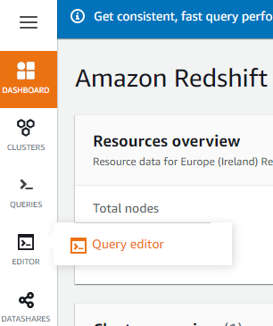
Now let’s see how to get started with Redshift. For querying both to Redshift-managed data and to external data in S3 (via Spectrum), a running cluster is required. The Redshift UI offers access to an SQL editor:

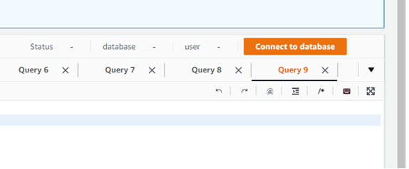
Once in the editor, connect to the database specified during the creation of the cluster by clicking the orange button in the upper-right corner:

It is also possible to create more databases in addition to the first one; you can connect to them the same way.

After connecting to a database, its schemas will appear in the Resources column, on the left side of the screen:

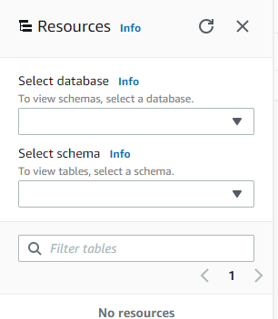
There is no need to specify a database in the queries unless it is a database other than the one you are connected to; we only need to specify the schema where the tables are. It is advisable to use schemas instead of creating tables directly if you are going to use Spectrum, because only external schemas can be queried through Spectrum.

Now that the introductions are over, let’s get down to our demonstration of how to use Redshift.

Hands-on Redshift

In this section, we will first explain how to import data into Redshift from S3 and create the tables with the corresponding distribution and sorting keys, and later how to use Spectrum to query external data in S3 directly. Finally, we will compare the results of both approaches (loading data internally in Redshift versus querying directly with Spectrum).

The dataset that we are using is the same one we used in previous articles in this series, i.e. the TPC-H dataset, of which we have three different versions as described in the introduction (CSV, Parquets without partitions, and Parquets with the two largest tables partitioned).

Local Tables (Redshift)

First, we start by loading the data internally into Redshift.

It is recommendable to load the dataset in a compressed format, like Parquet, because it is faster than raw data like CSV. We should also consider that Redshift does not support Hive partitions and will not read the fields in the name of the folders (e. g.: l_shipdate=1992-08-02). If your dataset is partitioned, you will have to add the partitioned fields as another column in your tables, so the easiest option is to load our second version, Parquets without partitions.

The structure of the data loaded into Redshift is key to optimising the queries that we will make, so we need to study the queries to select the best combination of distribution and sort keys. But before we do that, if we look at the schema of the dataset, we can distinguish a star flake schema, with lineitem as a union between the tables related to part and supplier, and orders and customer.

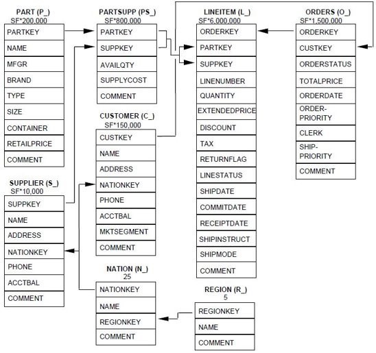
Most of the queries we are going to run (a subset of the queries defined in the TPC-H specification) use JOINs to link the tables, so we are going to use the identifiers of each table (orderkey, partkey, suppkey…) as distribution keys.

Another common trait in the queries is the use of date filters; in most cases the date is used in ‘between’ filters. To ease the reading of the data and allow Redshift to skip data blocks, data is sorted by date, with the same columns as the partitioned dataset, l_shipdate and o_orderdate.

Here is the code we used to create the lineitem table:

/* LINEITEM TABLE */   
CREATE TABLE tpc_db_cluster.lineitem( 
	l_orderkey BIGINT NOT NULL distkey, 
	l_partkey BIGINT,
    	l_suppkey int,  
	l_linenumber int,   
	l_quantity float,  
	l_extendedprice float,  
	l_discount float,  
    	l_tax float,  
	l_returnflag varchar(1), 
        l_linestatus varchar(1),  
        l_shipdate date NOT NULL, 
        l_commitdate date, 
        l_receiptdate date,
        l_shipinstruct varchar(25),
        l_shipmode varchar(10),    
        l_comment varchar(44)      
)   
SORTKEY(   
        l_shipdate,   
        l_orderkey   
); 

Once the table is created data can be loaded into the cluster with the copy command:

copy tpc_db_cluster.lineitem  
from 's3://redshift-evaluation/tpc-h-100gb-opt/lineitem/'  
iam_role 'arn:aws:iam::999999999999:role/Redshift_access' 
FORMAT AS Parquet; 

If the dataset is in CSV format the syntax would be different in the last line; it would be:

copy tpc_db_cluster.lineitem  
from 's3://redshift-evaluation/tpc-h-100gb-opt/lineitem/'  
iam_role 'arn:aws:iam::999999999999:role/Redshift_access 
CSV;

After loading the data into Redshift, to ensure that the distribution and sorting keys work as specified, the vacuum command should be executed on each table:

vacuum full tpc_db_cluster.lineitem;  

Now that the data is correctly stored in the cluster, you can start querying!

After running a query in the UI, the results are shown below the text field, in the Query results tab. They appear automatically when the execution finishes. The elapsed time and the query identifier are also shown, but disappear between executions.

The elapsed times of previous queries can be seen in the Query history tab, on the upper side of the page. If more information is needed, we recommend using queries to internal system tables of Redshift, such as ‘stl_query’, which stores metadata related to executed queries. Here is an example of a query with this table:

/* General information (id, text, time, user...) about last queries */   
select *   
from   
    stl_query a,   
    stl_utilitytext b   
where   
    a.pid = b.pid   
    AND a.xid = b.xid   
order by   
    query desc; 

There are more system tables to help with managing Redshift; more information can be found in the AWS documentation.

As we commented above, if you have a running Redshift cluster and want to perform some ad hoc queries to S3 without loading them into the cluster, you can use external tables with Redshift Spectrum. This is what we will demonstrate next with the same dataset.

External Tables (Spectrum)

Before we can query external data with Spectrum, there are some actions that we need to take. First, an external schema in Redshift must be created, that points to a database defined in the catalogue:

CREATE external schema tpc_db  
from data catalog  
database 'tpc_db'  
iam_role 'arn:aws:iam::999999999999:role/Redshift_access'  
CREATE external database IF NOT EXISTS; 

In the example above, we create the external schema tpc_db in Redshift that points to a database with the same name in the AWS Glue Data Catalog. Note that if the database in the catalogue does not exist, the above command will create it.

If the database already exists, then the tables in it have probably been defined already – this was the case for us since we were reusing the catalogue database we created in our previous blog post related to Athena, which also uses the same catalogue – the tpc_db database contains the 8 tables in CSV.

Note that if the database did not exist, then it would not contain tables and we would need to add them now. In that case, we could create tables from Spectrum as we do in Athena. Below you can see how to create a table from CSVs:

/* ORDERS TABLE */  
CREATE external TABLE  tpc_db.orders(  
	o_orderkey BIGINT,  
	o_custkey BIGINT,  
	o_orderstatus varchar(1),  
	o_totalprice float,  
	o_orderdate date,  
	o_orderpriority varchar(15),  
	o_clerk varchar(15),  
	o_shippriority int,  
	o_comment varchar(79)  
)  
ROW FORMAT DELIMITED  
FIELDS TERMINATED BY '|'  
STORED AS textfile  
LOCATION 's3://redshift-evaluation/tpc-h-100gb-opt/orders/';  

We also created an external schema for the Parquet tables without partitions. As with the CSVs, the tables were already defined, but if we needed to define them in Spectrum we could do it like this:

/* ORDERS TABLE */  
CREATE external TABLE  tpc_db_opt.orders(  
	o_orderkey BIGINT,  
	o_custkey BIGINT,  
	o_orderstatus varchar(1),  
	o_totalprice float,  
	o_orderdate date,  
	o_orderpriority varchar(15),  
	o_clerk varchar(15),  
	o_shippriority int,  
	o_comment varchar(79)  
) 
STORED AS Parquet  
LOCATION 's3://redshift-evaluation/tpc-h-100gb-opt/orders/';

Finally, we also created an external schema for the partitioned dataset (only the two largest tables are partitioned). As with the schemas for the CSVs and the Parquets without partitions, the tables were already defined. However, if we needed to define them in Spectrum, we could do it like this:

CREATE external TABLE  tpc_db_opt_part.orders( 
	o_orderkey bigint, 
	o_custkey bigint,
    	o_orderstatus string,
	o_totalprice decimal(18,2),
	o_orderpriority string,
	o_clerk string,
	o_shippriority int,
    	o_comment string
) 
PARTITIONED BY (o_orderdate date) 
STORED AS Parquet  
LOCATION 's3://redshift-evaluation/tpc-h-100gb-opt/orders-part/'; 

If you are defining the table in Spectrum, bear in mind that to query partitioned data, partitions must be added one by one, up to a maximum of 100 at a time:

alter table tpc_db_part.orders 
add partition(o_orderdate='1998-01-01') 
location 's3://redshift-evaluation/tpc-h-100gb-opt/orders-part/'; 

If you have a lot of partitions, it would be better to think about an alternative. In our case, we just used the table created with Athena that already had the metastore updated with all the partitions.

Once the three external schemas have been defined (one for each dataset version) and all the tables too, we are set to query external data via Spectrum.

When running a query with Spectrum, results and execution times are shown as when working with internal data. This time, though, there is another important metric with Spectrum, the size of the data scanned, because the amount charged depends on it. We have not been able to see this value anywhere in the UI, but there is a table with information of executed queries from Spectrum to S3 named svl_s3query_summary.

The following example shows the ID of the last queries with the time elapsed since they were queried, and the amount of data scanned in GB (the original value is in bytes):

/* SPECTRUM - Metrics from last queries */   
select query, sum(elapsed)/1000000.0 as elapsed, sum(s3_scanned_bytes)/(1024.0*1024.0*1024.0) 
as scanned   
from svl_s3query_summary   
group by query   
order by query desc;  

Note there will be no costs for reading from this metadata table because it is internal, located inside the Redshift cluster.

Results Analysis

Next, we ran the same set of queries for the four different scenarios as we did in our previous blog post. The first scenario is when we have loaded the dataset internally into Redshift and used distribution and sort keys. The other three scenarios refer to the use of Spectrum to query the datasets in S3 in its three versions (CSV, Parquets without partitions, and Parquets with the two largest tables partitioned).

As in Athena, the use of Parquet with Spectrum lowers query time and the data scanned. However, if we compare the results between Spectrum and queries with the Redshift internal data, large queries that use filters or multiple JOINs take advantage of the distribution and sorting of the data, so using the internal data generally offers better performance. Some queries might be faster with Spectrum when there are aggregates and no JOINs, or with filters that are not considered as the distribution or sorting fields.

Usually, importing the data into the Redshift cluster leads to more performant queries due to its structure optimisation with the sorting and distribution keys. However, a bad implementation of these, or running queries that do not leverage them, will lead to bad performance, with Spectrum giving better results.

RedShift and Tableau Connection

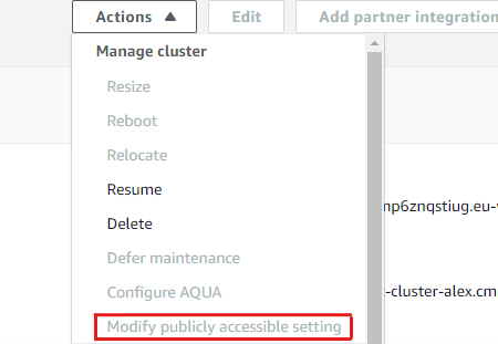
The connection between Redshift and Tableau Desktop can be tricky. Before going into detail, it is necessary to check that the Redshift cluster is accessible from the outside: this can be changed by stopping the cluster and selecting ‘Modify publicly accessible setting’ from the Actions dropdown menu in the Cluster page:

The installation of some drivers may also be necessary. Following the steps in this official Tableau web page, you will be able to prepare everything necessary to connect Tableau to Redshift.

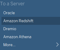
Once ready, make sure you have restarted Tableau after the installation. And on opening a new data source to a server, Amazon Redshift will appear among all the possibilities:

A window appears asking for information about the cluster and some credentials to connect to it:

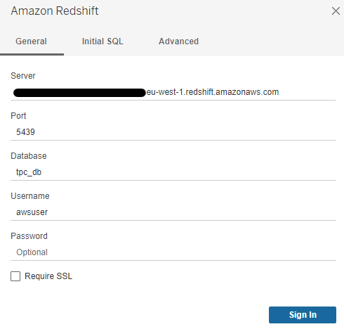
The server URL can be found in Redshift > Your Cluster > Endpoint, in the General Information box:

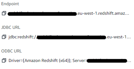
The port, the database name and the admin username are the same as specified during the creation of the cluster, and they remain visible in the Database configurations box, below the General information box.

There is no difference between using Tableau with Redshift Spectrum or Redshift. The connection is to the cluster to monitor the metrics, though the svl_s3query_summary table must be used.

Similarly to Athena, the use of Spectrum via reporting tools is discouraged unless you really know what you are doing, because there could be an increased cost when running queries, as Tableau has its own query planning. The use of the cluster and the internal Redshift data, though, does not have any of these drawbacks. However, as we also commented in the previous article, Tableau doesn’t deal with JOINs performantly, so before making any operation it is very advisable to create intermediate tables or views with the JOINs already made, or use aggregated tables.

Conclusion

Amazon Redshift can be an excellent solution for data warehousing, offering the opportunity to use Spectrum to query data in S3 without having to load it. Though Spectrum queries may not be as fast as those that query equivalent internal data (if distribution and sort keys are well implemented), there are cases in which it may be particularly useful if you cannot or do not want to load the data into the cluster.

Some aspects worth considering are the necessity of learning about the way Redshift structures data with sort keys and distribution styles to always find the best way to use them, plus the need to carry out maintenance tasks to keep up performance.

The benefits we would highlight are:

• Highly and easily scalable.
• Supports a wide range of structured and semi-structured data formats.
• Data may be rapidly loaded as Redshift uses Massively Parallel Processing (MPP).
• Supports external data querying with Spectrum.

However, there are also some things to consider:

• Requires understanding of sort keys and distribution styles.
• Partitioned data is tricky to load.
• A running Redshift cluster is needed to use Spectrum; creating a cluster only to run ad hoc queries is not necessary because Athena is designed specifically for that purpose.
• Like many cloud projects, Redshift is not recommended for small projects (1 node), because it cannot leverage the distribution keys.

We have seen that Redshift is a great data warehouse solution if you know how to design the corresponding sort and distribution keys properly. Although it might not be the best option for small projects, for large projects where there are many concurrent users running complex queries and using BI tools, it is a recommended choice. The combination of S3, Redshift and Athena is what AWS proposes as a data lakehouse.

Having said this, Redshift is not the only data warehouse choice available in the market, nor is the combination with S3 and Athena the only data lakehouse alternative: there are a few more as we will see in the coming blog posts in this series.

One alternative could be Snowflake, which is a data warehouse that allows loading the data into its internal system to optimise queries, and it also supports querying directly to external sources such S3. Snowflake also embraces the data lakehouse concept. In the next blog post of this series, we will explain how Snowflake works and its benefits, so stay tuned!

For more information on how to get the most out of Redshift, simply contact us! We will be happy to help and guide you into taking the best decision for your business.

The blog series continues here.