30 Aug 2023 How to Create Custom Machine Learning Models in Oracle Analytics
In our previous Oracle Analytics Machine Learning (ML) blog post we introduced the tool, saw how to install it, how to prepare data, and how to use the ML module, as well as taking a look at custom scripting. In today´s blog post we´ll look at some detailed know-how about creating custom models in Oracle Analytics Server (OAS).
We just finished a project for a customer who wanted to automate their ML process using OAS ML capabilities. The customer was extracting the data manually from OAS, importing it locally as an Excel file, then running the Python scripts whenever they wanted to get the results, a time-consuming task even on a small scale. As the customer needed to scale it up, they decided to leverage the Oracle platform that was already in place to automate certain parts of the process to save both time and resources.
The entire automation process can be summarised into:
- Setting up the environment and installing Python libraries.
- Adapting Python scripts for Oracle.
- Creating data flows for data transformation, training, applying, and validating the model.
- Building reports.
- Scheduling data flows.
We will focus on the first two steps, as this is where we encountered the most issues and also experienced a lack of documentation and guidance.
Installing Python Libraries in OAS
We might need some Python libraries in a Python script that are not installed in OAS by default, so here’s a step-by-step guide on how to install them:
Please note that the paths mentioned will be slightly different on your machine.
- Set the below variables’ value for the OAS instance (specific for each instance):
DOMAIN_HOME=/u02/OAS/config/domains/oasbi
ORACLE_HOME=/u02/OAS/oas_5.9 - Check if python3-pip is already installed. If not, install it, as you´ll need it to install other libraries:
sudo yum install python3-pip
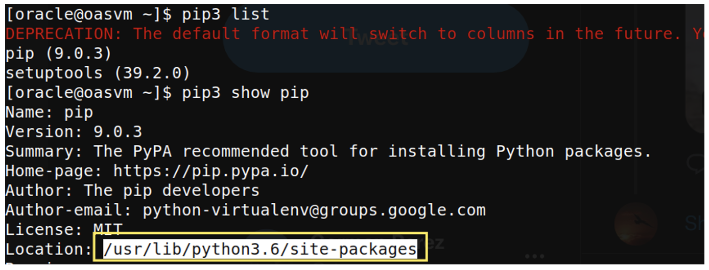
- Find out where the pip package folder resides:
pip3 show pip

Figure 1: Pip package location
- Copy the pip folder into the OAS Python packages folder:
cp -r /usr/l ib/python3.6/site-packages/pip $ORACLE_HOME/bi/modules/oracle.bi.dvml/lib/python3.5/site-packages
- In preparation for the installation of the package:
- Export the value for the environment variable LD_LIBRARY_PATH:
exportLD_LIBRARY_PATH=$LD_LIBRARY_PATH:$ORACLE_HOME/bi/modules/oracle.bi.dvml/lib
LD_LIBRARY_PATH is an environmental variable used to tell dynamic link loaders where to look for shared libraries for specific applications.
- Copy the Makefile in the Python installation folder:
cp /usr/lib64/python3.6/config-3.6m-x86_64-linux-gnu/Makefile
$ORACLE_HOME/bi/modules/oracle.bi.dvml/lib/python3.5/config-3.5m
The Make utility is a software tool for managing and maintaining computer programs consisting of many component files. It automatically determines which pieces of a large program need to be recompiled, and issues the necessary commands to do so. Make reads its instruction from the default Makefile (also called the descriptor file). Essentially, Makefiles serve to automate software building procedures and other complex tasks, complete with their dependencies.
- Export the value for the environment variable LD_LIBRARY_PATH:
Install the missing library for the OAS Python instance, for example geopy:
$ORACLE_HOME/bi/modules/oracle.bi.dvml/bin/python3.5 -m pip install geopy
Adapting Python Scripts to Oracle
When dealing with a functional Python script, we need to embed it into XML, because that´s the only format Oracle accepts. This XML file has some tags that are mandatory, and others that are optional – the initial tag is the script tag, and every other tag is an element of the script tag. Important sub-elements are:
- Scriptname – it should be the same as the name of the script.
- Group – which group of algorithms yours belongs to (Machine Learning (Supervised) or Machine Learning (Unsupervised)).
- Algorithm – state which algorithm is being used.
- Scriptdescription – description of the script, mustn’t have extra spaces (otherwise script couldn’t be uploaded in OAS)
Instead of adding it like this…:<scriptdescription> <![CDATA[ This script performs classification and regression with Random Forest on the input data.The input is a data frame with target, attribute1, attributes2....The output includes model object and model descriptive data. ]]> </scriptdescription>
…remove the extra spaces:
<scriptdescription><![CDATA[This script performs classification and regression with Random Forest on the input data.The input is a data frame with target, attribute1, attributes2....The output includes model object and model descriptive data.]]></scriptdescription>
- Class – custom.
- Type – when training a model it’s create_model, when applying it it’s apply_model.
- Inputs – input parameters.
- Outputs – output parameters.
- Options – options you can define in your script, either mandatory or optional. Here you define all the variables that will be used in the Python script.
- Scriptcontent – the Python script. When training a model you have to define the obi_create_model(data, columnMetadata, args) function, and when applying the obi_apply_model(data, model, columnMetadata, args)
When we started working on the customer project mentioned above, we realised that the publicly available documentation was very limited for custom predictive modelling. There are examples of custom scripts in the Oracle Analytics Library, and the 2018 blog on blogviz. During the project we encountered many problems and challenges we needed to overcome, and here we are going to look at some of them.
Custom Training Script
When creating the custom training script, we didn’t need to use input and output parameters. The input dataset is automatically sent as the input argument in the obi_create_model function, while the output of the script, model and datasets are returned in the function itself. All the variables needed for training the model are defined through the options tag.
As mentioned before, the last XML element is scriptcontent where the Python script is placed. First the Python libraries are imported, then the function obi_create_model(data, columnMetadata, args) needs to be defined with input arguments:
- data – the training dataset that is defined in the data flow.
- columnMetadata – the metadata of the input columns.
- args – arguments that are defined in the <options> tag.
We can divide the content of the function into segments:
- Reading optional parameters into variables.
- Cleansing and dataset manipulation.
- Training and creating the model.
- Adding related datasets: generating testing outputs, calculating metrics.
Reading Optional Parameters into Variables
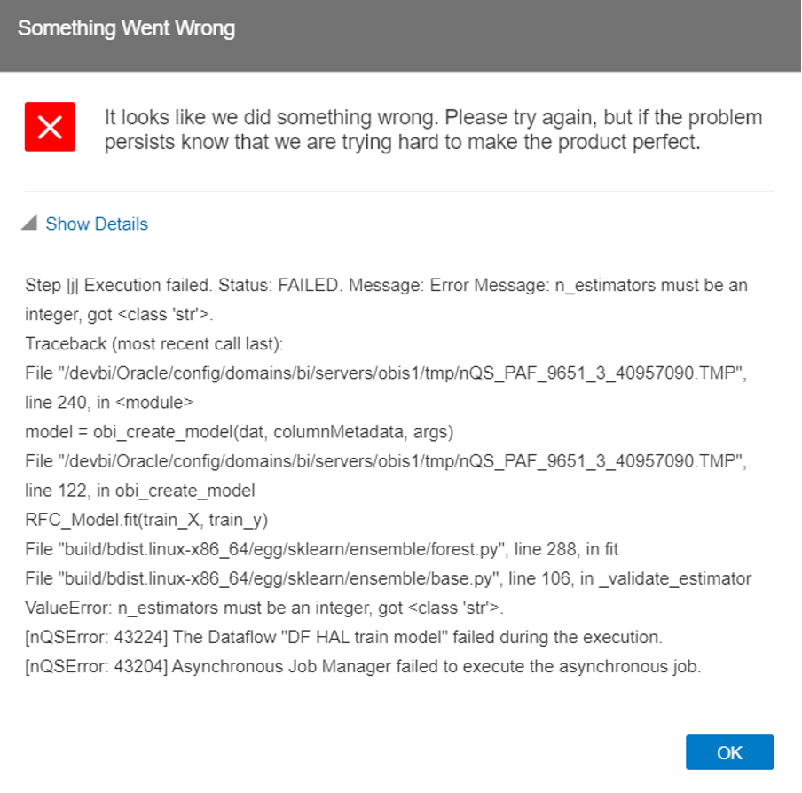
During the project we noticed some issues with variables: if a variable has to be numeric, it needs to be converted to a number while reading it to a Python variable, as all the variables are saved as strings by default. If not, the following error appears:

Figure 2: Data type error
Let’s say we have defined target and num_of_trees variables in the options tag; we should read them like this:
target = args[‘target’]
numOfTrees = int(args[‘num_of_trees’])Cleansing and Dataset Manipulation
Now that the variables are ready, we should clean the dataset and make transformations: Oracle have built their own datasetutils module for this purpose, and if we check their example of the custom script, we’ll see that it’s being used. The location of the script is:
/u02/OAS/oas_5.9/bi/bifoundation/advanced_analytics/python_scripts/obipy/obisys/
where you can check its definition and perhaps use some of the functions, like:
- fix_column_names (column_names).
- fill_na (dat, max_null_percent=50, numerical_impute_method=’mean’, categorical_impute_method=’most frequent’).
- features_encoding (dat, targetname=None, targetMappings=None, encoding_method=”indexer”, type = “classification”).
To use the module you need to import it to the Python script with:
from obipy.obisys import datasetutils
As the functions fix_column_names and fill_na are described in the Oracle Analytics Library, we will only mention features_encoding. In our project we used a classification algorithm, so the target variable mapping needed to be defined. Another thing that turned out to be very important was the listing of the features and using encoded data explicitly defined by categorical and numerical features throughout subsequent sections of the script:
targetMappings = {'Yes':1, 'No':0}
data, input_features, categorical_mappings = datasetutils.features_encoding (dat=df,targetname=target, targetMappings=targetMappings, encoding_method="indexer", type="classification")
features = list(input_features['categorical']) + list(input_features['numerical'])
features_df = data[features]
This way of defining the data fixates the order of the variables (features); we will return to this point in the apply script.
Training and Creating the Model
At this point, the dataset should be split into a training set and a test set. Then the model is trained using the desired algorithm along with the variables from the options tag. After the creation of the model, a dictionary is defined containing the model and its parameters, and saved as a pickle object, so it can be accessed via a reference name during subsequent applications, like this:
pickleobj={'RandomForestClassification':RFC_Model}
d = base64.b64encode(pickle.dumps(pickleobj)).decode('utf-8')
In order to save the model in OAS, it needs to be defined using the Oracle Model module. Required attributes can be set like this:
model = Model()
model.set_data(__name__, 'pickle', d, target)
model.set_required_attr(required_mappings)
Adding Datasets to the Quality Tab
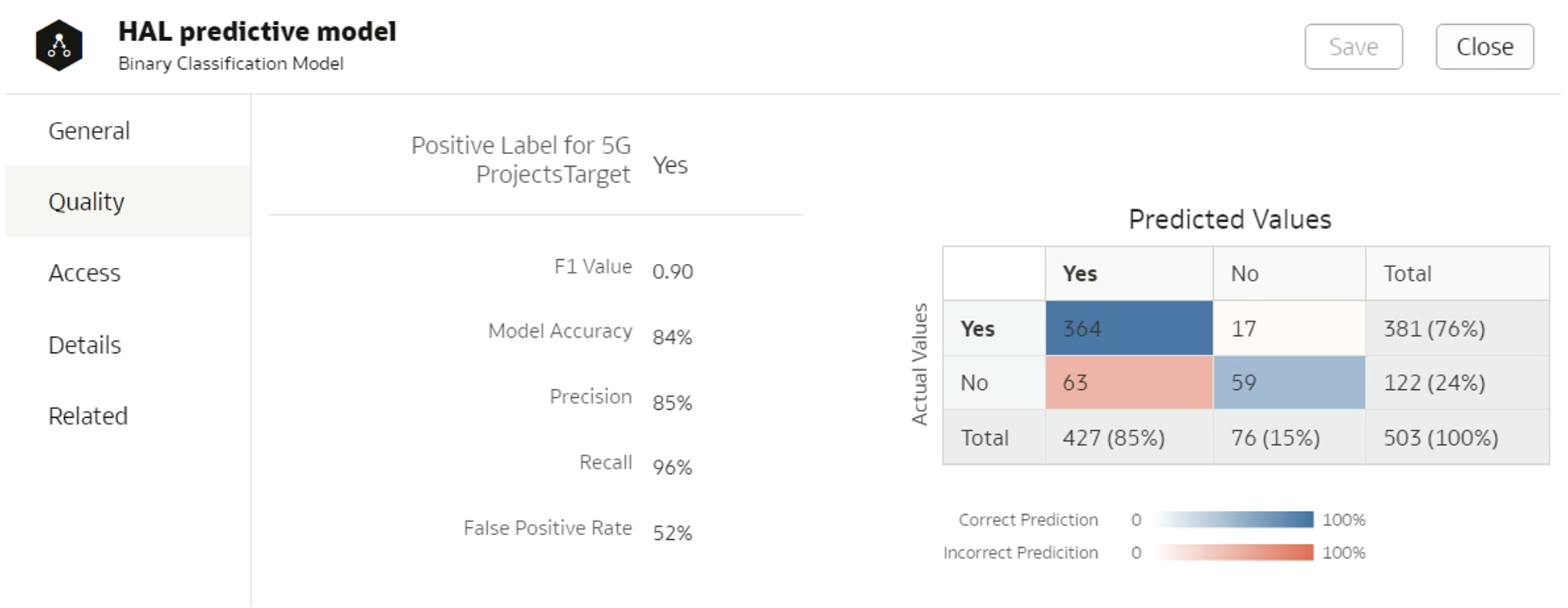
Once the model has been generated, we can inspect it and check its quality. To get quality-related insights like those shown in Figure 3 below, it’s important to set a class tag for the model, and a positive class in the case of binary classification algorithms:
model.set_class_tag("BinaryClassification")
model.set_positive_class("Yes")
Figure 3: Quality tab
The class tag for a classification model can either be “BinaryClassification” or “MultiClassification”, and for regression the class is “Numeric”. Diverse algorithm types correspond to different datasets that appear in the Quality tab – regression should display a “Residuals” dataset, classification a “Confusion matrix” dataset, and both should have a “Statistics” dataset. There are specific rules governing the display of datasets in the Quality tab:
1. Set the appropriate class when defining the model, as described above.
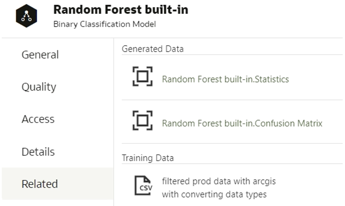
2. Save the data in the data frame object. The dataset´s header must contain the same columns as the header of the built-in model dataset; you can find out the names of the columns if you create a data flow for training the data and choose a built-in algorithm. When inspecting the model, generated data appears in the Related tab:

Figure 4: Related tab and datasets
Click on the generated data to find the column names:

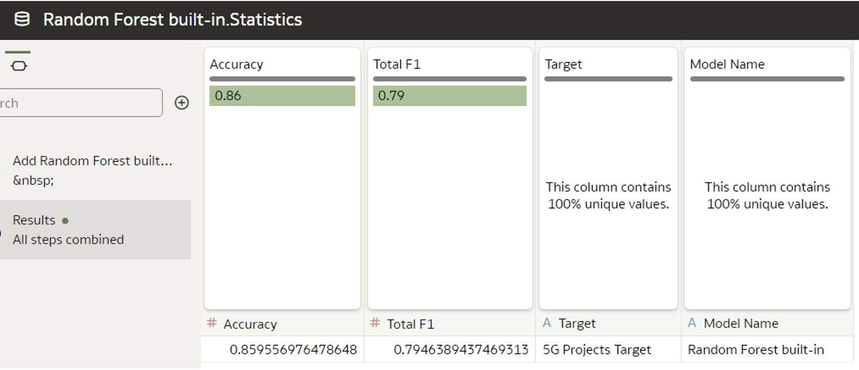
Figure 5: Header of built-in generated dataset
The custom model metrics should be named in the same way, although the order is not important. While there´s the option to include more metrics than the foundational ones, note that only the pre-defined metrics will appear in the Quality tab.
3. Dataset mapping can be defined, including column names, data types, and aggregation functions for each column. Nevertheless, this is optional, and you can assign None; Oracle will autodetect it.
4. Add the output dataset using a built-in function:
f1_df = pd.DataFrame({'Accuracy': [accuracy], 'Total F1': [f1], 'Precision': precision_positive, 'Recall': recall_sensitivity, 'FPR': fpr})
f1_mappings = None
f1_ds = ModelDataset("Statistics", f1_df, f1_mappings)
model.add_output_dataset(f1_ds)
In addition to the datasets visible in the Quality tab, any other dataset can be generated and will be displayed in the Related tab; to do so, follow Steps 3 and 4.
Custom Apply Script
When the training script is ready, we should adapt the corresponding script for model application. Here, it’s important to define the output columns in the <outputs> tag; these are new calculations that we want to retrieve. Input data can be retrieved only by concatenating it to the results.
We can divide the content of the function obi_apply_model(data, model, columnMetadata, args) into segments:
- Loading the custom prediction model.
- Cleansing and manipulation of the dataset.
- Prediction.
- Generating output.
Loading the Prediction Model
The model is fetched based on the tag assigned in the training script:
pickleobj = pickle.loads(base64.b64decode(bytes(model.data, 'utf-8')))
RFC_Model=pickleobj['CustomRandomForestClassification']
Cleansing and Manipulation of the Dataset
The prediction dataset should be prepared in the same way as the training set. Once again, we list the features after encoding and use this encoded data in the script, which is explicitly defined using categorical and numerical features.
data, input_features, categorical_mappings = datasetutils.features_encoding (df, None, None, encoding_method="indexer", type = "classification")
features = list(input_features['categorical']) + list(input_features['numerical'])
df = data[features]
If we don´t do this and instead use the data output from datasetutils.features_encoding, we will get different results each time we run the script for value prediction. This is because the variables in the features_encoding are in a random order in each iteration and the model calculates the results based on the position of the variable, not its name.
Prediction and Output
Now, the last task is to predict the values and to concatenate the input dataset in the following way:
y_pred=RFC_Model.predict(df)
y_pred_prob = RFC_Model.predict_proba(df)
y_pred_df = pd.DataFrame(y_pred, index=df.index, columns=['predictedValue'])
y_probs_df = pd.DataFrame({"prob0" : y_pred_prob[:,0], "prob1" :
y_pred_prob[:,1]}, index=df.index)
output = pd.concat([y_pred_df, y_probs_df, input_data], axis=1)
Error Handling
The tool’s error handling is not optimal and often gives general errors, so we needed a workaround to catch them:
- We added a sleep command in the train/apply script (whichever was failing) to catch the temporary files created when the script is triggered:
import time
time.sleep(120)
- Inspecting logs:
cd /u02/OAS/config/domains/oasbi/servers/obis1/logs
tail obis1.out
This command provides the full error and also contains the name of the temporary file where it occurred, ex. nQS_PAF_15199_1_31114775_3.TMP. The TMP file contains the entire code that is being compiled: custom Python script and Oracle add-ons.
- Temporary files:
cd /u02/OAS/config/domains/oasbi/servers/obis1/tmp
ls -lptr
This command will list all the files in the path with their details. We copied all the files relevant to our process (one of the files would be the TMP file, and the rest can be recognised by having the same timestamp) by executing:
cp nQS_PAF_15199_1_31114775.TMP nQS_PAF_15199_1_31114775_copy.TMP
This allowed us to inspect the code and the input/output files. - For simplicity and to save time, we would make the changes on the copied TMP script and run it in Linux, to avoid uploading the custom script to the tool:
export PYTHONPATH=/u02/OAS/oas_5.9/bi/bifoundation/advanced_analytics/python_scripts
export LD_LIBRARY_PATH=/u02/OAS/oas_5.9/bi/modules/oracle.bi.dvml/lib
cd /u02/OAS/config/domains/oasbi/servers/obis1/tmp
/u02/OAS/oas_5.9/bi/modules/oracle.bi.dvml/bin/python3.5 /u02/OAS/config/domains/oasbi/servers/obis1/tmp/nQS_PAF_15199_1_31114775_copy.TMP
When making a copy of the TMP and input files, be sure to rename the input.xml and .csv files back to their original names, as TMP references those.
Iterating through these steps, we solved all of the errors!
Other paths that could be of help are:
- The location for storing external subject areas (XSA); created models and datasets are saved here:
/u02/OAS/config/domains/oasbi/bidata/components/DSS/storage/ssi/ - The main path for algorithm libraries (like linear_regression, random_forest, etc.):
/u02/OAS/oas_5.9/bi/bifoundation/advanced_analytics/python_scripts/obipy/tools - The path for libraries used by the main algorithm libraries (like RandomForest, Predictor, CrossValidator, etc.):
/u02/OAS/oas_5.9/bi/bifoundation/advanced_analytics/python_scripts/obipy/obiml
Tips and Tricks
- To upload a new version of a custom script, the old version (with the same name) must be deleted from the tool.
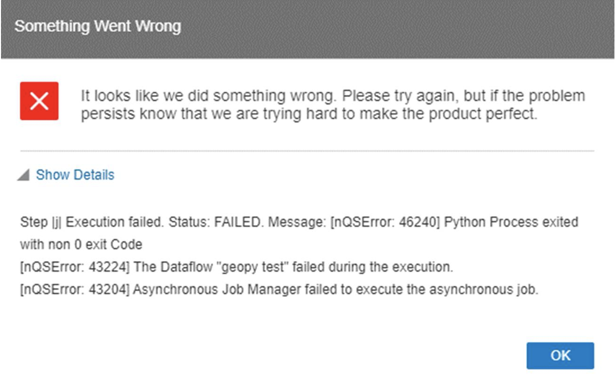
- Ensure consistent indentation throughout the entire XML files, including both the tags and the Python scripts, as an inconsistent use of indentation, such as mixing spaces and tabs, can lead to general errors. We faced an issue with this because we initially used a portion of code from Oracle’s custom script example, which employed spaces for indentation, but when we added new code we used tabs for indentation, leading to inconsistencies:

Figure 6: General error
We solved this issue with the error handling workaround described above.
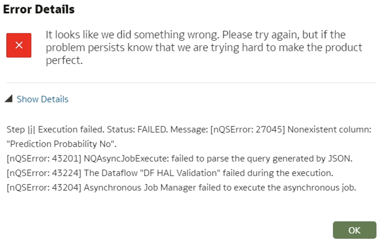
- When a column is removed from the data flow for training/applying the data, an error pops up saying that the column is missing. To avoid this, you need to delete the previously created model, sign out/sign in, train and apply the model again.

Figure 7: Error details for non-existing column
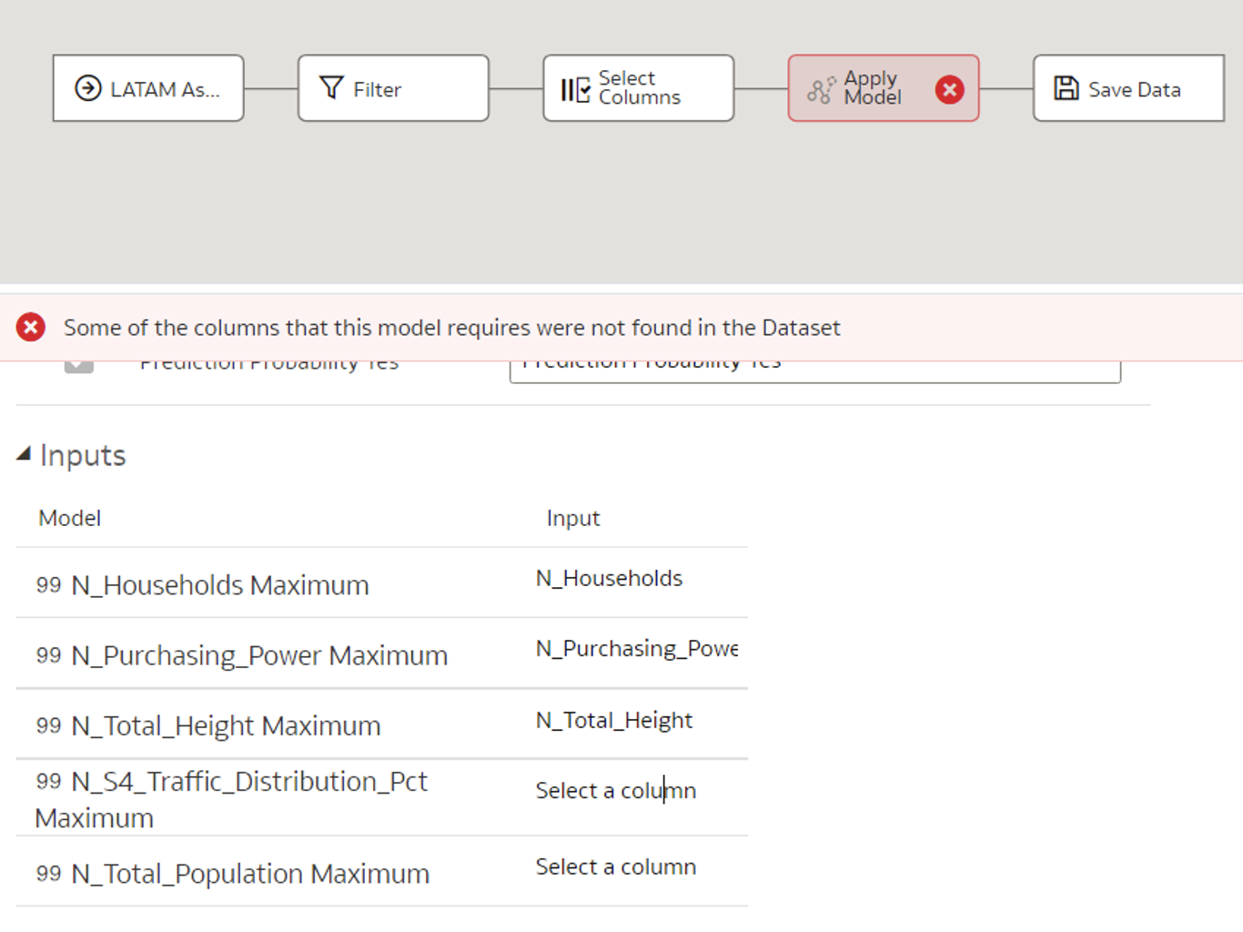
- If the input columns are named differently when applying the model compared to when it was initially created, those columns must be mapped manually:

Figure 8: Mapping columns with different names manually
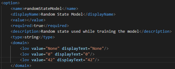
- If the columns added as input/output/options are of string data type and the domain is defined, then the attributes of the tag must be defined:

Figure 9: Domain tag
Conclusion
In our case, the key to a successful OAS ML implementation was access to the server, as without checking the logs in the server background it would have been impossible to debug any of the issues. The main reason for this is poor error handling and sparse documentation.
Another difficulty is platform dependency – if you are following Oracle custom script examples, there are references and calls to different built-in Oracle functions, so you can’t simply take Python code and run it locally to debug. These functions are also inaccessible if you don’t have server access, but a workaround for this is to install Oracle Analytics Desktop which allows you to access datasetutils.py and other useful scripts from your computer.
On a more positive note, it was a very interesting research and development experience, and it was amazing to see that you can build any predictive model using Oracle. We hope this blog will help you with building your own predictive model in OAS!
If you´ve got any queries or questions about any Oracle products, or if you´d just like to see how they can be leveraged to meet your needs, get in touch with our team of certified professionals!

- Set the below variables’ value for the OAS instance (specific for each instance):