29 Jul 2021 Integrating Cloudera with Dataiku and Power BI for Real-time AI/ML using NiFi and Kafka (Part 1/2)

In our two previous articles (one and two) we explained how to install NiFi (aka Cloudera Flow Management in the Cloudera stack) in a CDH (Cloudera Distribution of Hadoop) cluster and how to integrate it with Kafka and Hive to build a real-time data ingestion pipeline, with and without Kerberos integration.

Now, we want to take it one step further, showing you how you can (fairly easily) integrate your flow with other tools to create a slick real-time visualisation of an AI model applied to streaming data.

Dataiku DSS (Data Science Studio) is an extremely powerful and user-friendly tool that allows users with all sorts of backgrounds to apply Machine Learning and Artificial Intelligence models to their data with just a few clicks.

Power BI, part of the Microsoft offering, is a well-known data-visualisation tool that offers, amongst its various features, the possibility to have real-time dashboards.

At ClearPeaks, we are experts in both of them. In this series of two blog articles, we will leverage these two tools and NiFi to apply a trained AI model to the data streaming from your Kafka topic and visualise it in a dashboard in real-time.

In this first part, we will have a look at the overall pipeline and deep dive into the first segment of the flow, from the Kafka topic generation to the application of a Dataiku Machine Learning (ML) model on the fly. In the second part, we will see how to handle the answer coming from the DSS API and how to pass it on to the Power BI visualisation.

For our demo, we are going to assume that you have:

• Running instances of NiFi and Kafka.
• A Dataiku DSS instance, with a running API node and expertise on creating Dataiku projects and deploying and consuming APIs.
• A Power BI instance with enabled access to Streaming Datasets.

1. Overview

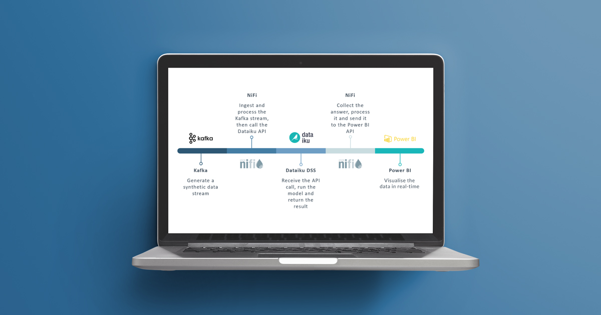
First of all, let us have an overview of the intended workflow.

On one side, we have our Kafka-Nifi platform. We will use it to stream and consume records from our cluster. These records will represent data about rental cars failures and maintenance information.

Then, we have Dataiku DSS. Dataiku offers a set of pre-made Artificial Intelligence cases which we can use as templates for our demonstrations. This comes in quite handy as you will be able to easily replicate our model. The good thing about Dataiku is that it also works as an API engine, which will allow us to take the records coming from Kafka and pass them to the AI/ML endpoint with a REST API call from NiFi, in order to predict their likelihood to fail based on the trained model.

Lastly – in our next blog entry – we will take the response from Dataiku and send it over to a Power BI Streaming Dataset, which will allow us to visualise our data and detect possible failures in real-time as the records flow through our pipeline.

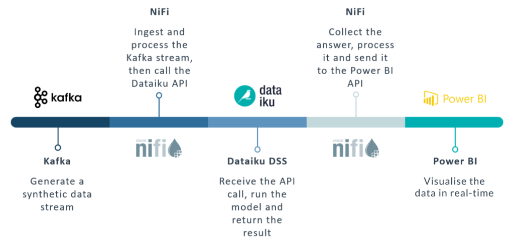
Figure 1: Overview of the full pipeline

2. The AI Model

As mentioned, Dataiku offers a number of AI/ML samples with which to experiment and deploy demonstrational models quickly. In our case, we picked the Predictive Maintenance template. Explaining how to create and use a Dataiku project falls outside the scope of this article (and is very easy), so let us look at how the project presents itself once it is created.

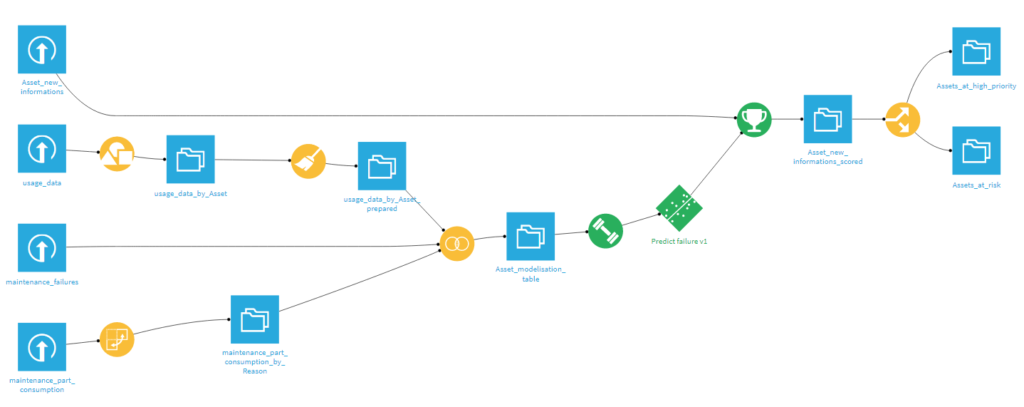
Figure 2: The Predictive Maintenance sample project in Dataiku

On the top left corner, we can see a dataset called Asset_new_information, which is the non-trained data that Dataiku provides you to effectively run an AI workflow. Essentially, that is what we want to replicate with our Kafka stream, in order to feed it to the API and get back a result which is based on the trained model.

We can edit or retrain our model if needed, and once we are satisfied, we deploy it to the API node (how to do so falls outside of the scope of the article, as well). We also make sure we enrich the API response by including at least the Asset column, so that we can recover the original asset to which the response belongs to, and push the NiFi flowfile down the pipeline to the correct Power BI dataset (as we will see in the next blog entry).  This can be done in the Enrichments and Advanced tabs of the API endpoint settings.

What we will obtain is an API endpoint with the following characteristics.

URL:

https://ai-dss.clearpeaks.com/api/public/api/v1/realtimedemo/maintenance/predict/

Payload example:

{
  "features": {
    "Asset": "A054380",
    "R417_Quantity_sum": 0,
    "R707_Quantity_sum": 3,
    "R193_Quantity_sum": 9,
    "R565_Quantity_sum": 0,
    "R783_Quantity_sum": 0,
    "R364_Quantity_sum": 0,
    "R446_Quantity_sum": 0,
    "R119_Quantity_sum": 0,
    "R044_Quantity_sum": 0,
    "R575_Quantity_sum": 0,
    "R606_Quantity_sum": 0,
    "R064_Quantity_sum": 0,
    "R396_Quantity_sum": 0,
    "R782_Quantity_sum": 0,
    "Time_begin_exploitation": 493,
    "Initial_km": 25854.262162562936,
    "nb_km": 398.83702767936484
  }
}

Response example:

{
  "result": {
    "prediction": "0",
    "probaPercentile": 3,
    "probas": {
      "0": 0.9745353026629604,
      "1": 0.02546469733703965
    },
    "ignored": false,
    "postEnrich": {
      "Asset": "A203778",
      "R417_Quantity_sum": "0",
      "R707_Quantity_sum": "3",
      "R193_Quantity_sum": "9",
      "R565_Quantity_sum": "0",
      "R783_Quantity_sum": "0",
      "R364_Quantity_sum": "0",
      "R446_Quantity_sum": "0",
      "R119_Quantity_sum": "0",
      "R044_Quantity_sum": "0",
      "R575_Quantity_sum": "0",
      "R606_Quantity_sum": "0",
      "R064_Quantity_sum": "0",
      "R396_Quantity_sum": "0",
      "R782_Quantity_sum": "0",
      "Time_begin_exploitation": "493",
      "Initial_km": "25854.262162562936",
      "nb_km": "398.83702767936484"
    }
  },
  "timing": {
    "preProcessing": 241,
    "wait": 113,
    "enrich": 25362,
    "preparation": 442,
    "prediction": 294609,
    "predictionPredict": 274452,
    "postProcessing": 157
  },
  "apiContext": {
    "serviceId": "realtimedemo",
    "endpointId": "maintenance",
    "serviceGeneration": " realtimedemo3850500813710946697"
  }
}

3. The Kafka Producer

As mentioned, we are going to replicate the data that the Dataiku model expects and feed it to NiFi via a Kafka topic.

To do so, we will first have to create a Python script to synthetically generate records with the required schema. The code to use is the one below:

import sys
import random
import datetime
import time

assets = ['A054380','A605703','A129740']

while True:
  for a in assets:
    myfile = open('car_record_'+a+'.log', 'a')
    Asset = a
    R417_Quantity_sum = (0 if random.randint(1,10)<=7 else random.randint(1,100))
    R707_Quantity_sum = random.randint(0,100)
    R193_Quantity_sum = random.randint(0,100)
    R565_Quantity_sum = (0 if random.randint(1,10)<=3 else random.randint(1,100))
    R783_Quantity_sum = (0 if random.randint(1,10)<=7 else random.randint(1,100))
    R364_Quantity_sum = (0 if random.randint(1,10)<=3 else random.randint(1,100))
    R446_Quantity_sum = (0 if random.randint(1,10)<=3 else random.randint(1,100))
    R119_Quantity_sum = (0 if random.randint(1,10)<=9 else random.randint(1,100))
    R044_Quantity_sum = (0 if random.randint(1,10)<=9 else random.randint(1,100))
    R575_Quantity_sum = (0 if random.randint(1,10)<=9 else random.randint(1,100))
    R606_Quantity_sum = (0 if random.randint(1,10)<=9 else random.randint(1,100))
    R064_Quantity_sum = (0 if random.randint(1,10)<=9 else random.randint(1,100))
    R396_Quantity_sum = (0 if random.randint(1,10)<=9 else random.randint(1,100))
    R782_Quantity_sum = (0 if random.randint(1,10)<=9 else random.randint(1,100))
    Time_begin_exploitation = random.randint(1,1000)
    Initial_km = random.uniform(25000,35000)
    nb_km = random.uniform(100,3000)

    myfile.write(
      Asset+','+ \
      str(R417_Quantity_sum)+','+ \
      str(R707_Quantity_sum)+','+ \
      str(R193_Quantity_sum)+','+ \
      str(R565_Quantity_sum)+','+ \
      str(R783_Quantity_sum)+','+ \
      str(R364_Quantity_sum)+','+ \
      str(R446_Quantity_sum)+','+ \
      str(R119_Quantity_sum)+','+ \
      str(R044_Quantity_sum)+','+ \
      str(R575_Quantity_sum)+','+ \
      str(R606_Quantity_sum)+','+ \
      str(R064_Quantity_sum)+','+ \
      str(R396_Quantity_sum)+','+ \
      str(R782_Quantity_sum)+','+ \
      str(Time_begin_exploitation)+','+ \
      str(Initial_km)+','+ \
      str(nb_km)+'\n'
    )
    
    myfile.close()
    time.sleep(1)

This code will generate three files, one for each of the assets:

• car_record_A054380.log

• car_record_A129740.log

• car_record_A605703.log

Of course, you can adapt the asset names as you prefer. In our case, we took 3 random names from the Dataiku set.

Then, as explained in our previous articles (for unsecure and kerberized clusters), we can chain the output of the files to a kafka-console-producer in order to send the messages to a previously created Kafka topic. In this case, since we have 3 files, we will create 3 producers (on 3 different sessions). Assuming the topic is called predictiveMaintenance and the files are within a folder called kafka_use_case, this would mean:

# cd kafka_use_case/
# export KAFKA_OPTS="-Djava.security.auth.login.config=/home/your_user/kafka_use_case/jaas.conf"                                                        
# tail -f car_record_A054380.log  2> /dev/null | kafka-console-producer --broker-list your_broker_node:9092 --topic predictiveMaintenance --producer.config client.properties

Once the Python script is running and our producers are started, they will feed the content of the asset files to NiFi, which will wait for it and pass it on as a sequence of flowfiles to the Dataiku API, after some manipulation.

4. The NiFi Pipeline

At this point, let us have a look at the NiFi pipeline.

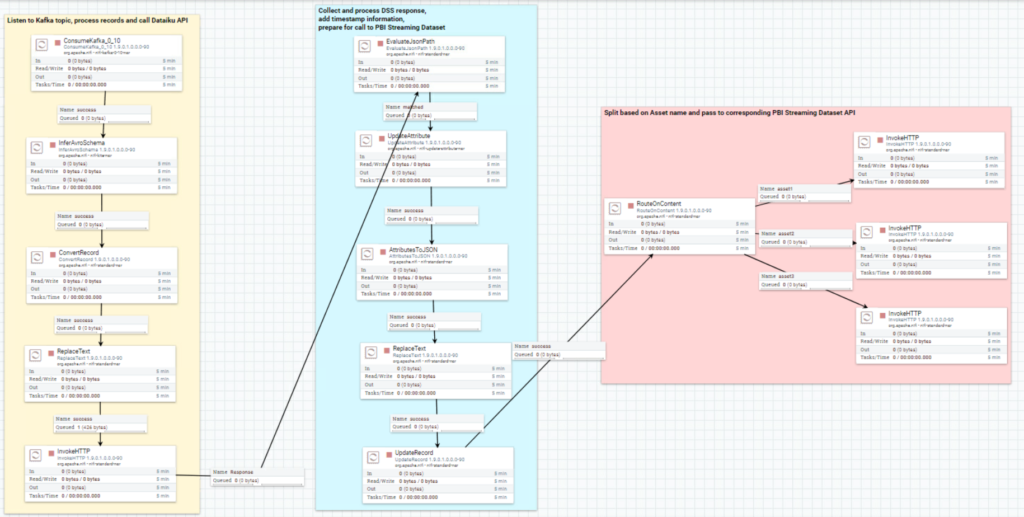
Figure 3: Overview of the complete NiFi pipeline

From the picture above, you can see that the pipeline is divided into three segments:

• The first pipeline segment listens to the Kafka topic, captures the messages coming from it, processes them so that they respect the JSON format required by the Dataiku model API, and passes them on to the endpoint with an HTTP call.
• The second part takes the response of the API call with results and probabilities alongside the original features, and furtherly processes the flowfile in order to prepare it for the Power BI Streaming dataset.
• Finally, the last part of the pipeline splits the flowfile based on the “asset”, which identifies the car described by a specific record. This step is sort of hardcoded, in the sense that we have to know what assets to expect before we are able to split the flowfile accordingly. Of course, there are better ways to handle this, but for our demo purpose the manual split was enough.

As anticipated, we will now look at the first segment in detail and explain the function and the settings of each processor. The remaining parts will be described in the second part of this blog series.

4.1. Process the Kafka stream and call the DSS API

Below we describe all the involved processors.

4.1.1. ConsumeKafka

In the ConsumeKafka processor, we setup our Kafka consumer by specifying the Kafka broker host and the topic name (predictiveMaintenance, in our case). Additionally, since our cluster is Kerberized, we also specify the SASL_PLAINTEXT protocol and a Kerberos Credential Service (for demonstration purposes, we used nifi’s credentials, but this can be adapted as required).

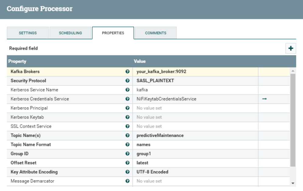
Figure 4: Hire Cost Analysis dashboard

For more details about the security settings on this processor, have a look at our previous article.

4.1.2. InferAvroSchema

This processor is responsible for detecting the schema of the incoming stream and storing it as an attribute of the flowfile. It will allow us to utilise this information in the next step, to convert the flowfile to a JSON array.

We need to specify the output destination of the detected schema, the format of the incoming stream and the names of the columns manually, since our data comes row by row without headers (other options are available as well). We also need to give the inferred schema a name.

When we choose flowfile-attribute as Schema Output Destination, NiFi will attach a new attribute to the flowfile, which will contain its schema and be used in the next step to perform the actual conversion.

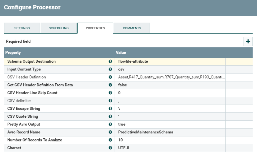
Figure 5: InferAvroSchema processor properties

4.1.3. ConvertRecord

As the name implies, this processor will convert the record from one format to another. Using the schema inferred in the previous step, we will turn our CSV flowfiles to JSON arrays. To do so, we need to define a Record Reader and a Record Writer controller.

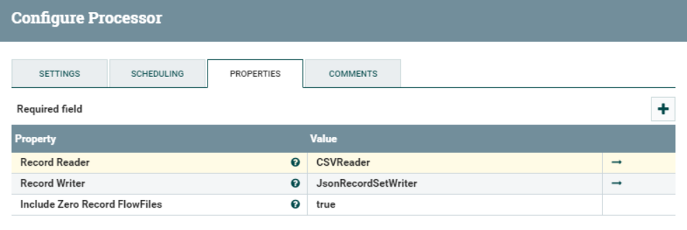
Figure 6: SDetails of the Convert Record processor

The Record Reader controller is configured as depicted below. We need to make sure that we are accessing the schema using the Schema Text property, and that this property’s value is ${inferred.avro.schema}. This is a NiFi variable that will hold the schema information inferred from the InferAvroSchema processor from the previous step.

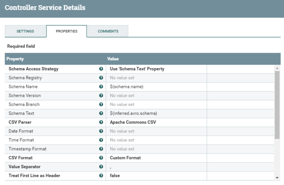
Figure 7: Settings of the Convert Reader controller service

For the Record Writer controller, we just need to make sure that the Schema Access Strategy is set to Inherit Record Schema. This will allow NiFi to automatically use the same schema used by the Record Reader to write the resulting JSON array.

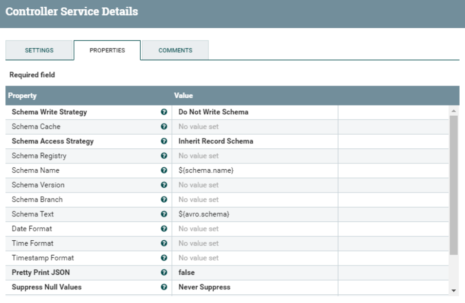
Figure 8: Settings of the Convert Writer controller service

4.1.4. ReplaceText

This processor allows us to replace parts of the text content of the flowfile using regular expressions. In this case, we need to wrap the whole JSON content in a new JSON property called features, to comply with the payload expected by Dataiku. Furthermore, we need to remove the square brackets of the JSON array.

This is done with the Search Value and Replacement Value illustrated below. Everything between the square brackets will be captured and represented by the $1 token you can see in the Replacement Value setting. The result will match with the payload required by the DSS API.

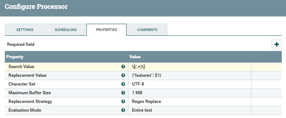
Figure 9: Details of the ReplaceText processor

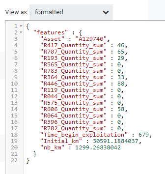
Figure 10: Flowfile format after the ReplaceText processor

4.1.5. InvokeHTTP

The InvokeHTTP is the last processor of this segment. It will take the incoming flowfiles (in JSON format) and send them to the Remote URL defined in its settings. This is the URL provided by Dataiku when creating the ML API.

We also have to specify the HTTP Method (POST), the content-type (application/json) and an SSL Context Service, since the Dataiku instance is secured with SSL.

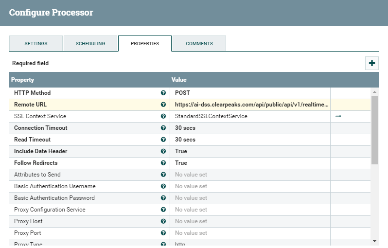
Figure 11: Settings of the InvokeHTTP processor

The SSL Context service controller allows us to tell NiFi the location of the keystore and truststore in the NiFi host(s), in order to correctly setup a secure communication with the DSS node. Of course, the keystore and truststore between the two parties need to contain the required certificates for this to happen.

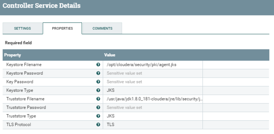
Figure 12: Details of the SSL Context Service controller

4.2. The response from Dataiku

Once the first segment of our pipeline is ready, we can start producing the stream and examining the queue coming out of the InvokeHTTP processor, to look at the response from Dataiku. Below, you can find the response to the request illustrated in Figure 10. We can see how we are receiving the predicted value, probabilities and statistical information about the prediction, the original features, and some additional metadata.

{
  "result": {
    "prediction": "0",
    "probaPercentile": 33,
    "probas": {
      "1": 0.27235374393191253,
      "0": 0.7276462560680876
    },
    "ignored": false,
    "postEnrich": {
      "Asset": "A129740",
      "R417_Quantity_sum": "46",
      "R707_Quantity_sum": "65",
      "R193_Quantity_sum": "29",
      "R565_Quantity_sum": "0",
      "R783_Quantity_sum": "0",
      "R364_Quantity_sum": "33",
      "R446_Quantity_sum": "88",
      "R119_Quantity_sum": "0",
      "R044_Quantity_sum": "0",
      "R575_Quantity_sum": "0",
      "R606_Quantity_sum": "58",
      "R064_Quantity_sum": "0",
      "R396_Quantity_sum": "0",
      "R782_Quantity_sum": "0",
      "Time_begin_exploitation": "679",
      "Initial_km": "30591.1884037",
      "nb_km": "1299.26838042"
    }
  },
  "timing": {
    "preProcessing": 370743,
    "wait": 1819,
    "enrich": 190846,
    "preparation": 179101,
    "prediction": 2022570,
    "predictionPredict": 838793,
    "postProcessing": 71
  },
  "apiContext": {
    "serviceId": "realtimedemo",
    "endpointId": "maintenance",
    "serviceGeneration": "v7"
  }
} 

Next Steps

In this article, we started looking at how to leverage the potential of 3 separate popular tools to build a neat real-time AI/ML pipeline. Specifically, in this first entry, we created a NiFi pipeline that captures data from a Kafka stream and sends it over to a Dataiku API endpoint, to apply a ML model on the fly. In the second entry, we will enrich the pipeline by consuming the response from Dataiku and pushing it to a PowerBI dashboard in real-time.

This specific scenario is probably not the most striking one (after all, it is “just” a simulation, and we are using a Dataiku template), but it should be enough to impress your users and is surely effective, considering the low amount of development and coding required. Once the door between NiFi and Dataiku is open, the possibilities are endless: you can build more ML models, more complex pipelines, or send the data to other visualisation tools such as Tableau.

Furthermore, we are not storing the data anywhere in our example, but in a real production scenario it might be wise (or even required) to save the incoming stream in HDFS or as a Hive table: this can be easily done in NiFi using the PutHDFS or the PutHiveStreaming processors (as seen here).

If coding and visualising your Machine Learning models interests you, make sure you have a look at this other blog post of ours, in which we describe and demonstrate the integration between Cloudera Data Science Workbench and Cloudera DataViz on an on-premise Cloudera Data Platform cluster.

If you have any questions, doubts, or are simply interested to discover more about Cloudera, Dataiku, Power BI, or any other data tool for that matter, do not hesitate to contact us at ClearPeaks. Our certified experts will be more than happy to help you and guide you in your journey through Business Intelligence, Big Data, and Advanced Analytics!