18 Oct 2023 IoT Framework for Data Simulation and Analytics with Azure and Cloudera: Part 2 – Data Analytics

This is the second blog post in our two-part mini-series to present and demonstrate an IoT framework that includes both data simulation and robust analytics. In the previous blog post, we first introduced the IoT framework, giving an overview of the whole solution, and then covered the data simulation component and provided a demonstration of how it works.

In this second part of the series, we’ll dive deeper into the analytical aspect, specifically focusing on the implementation with Cloudera Data Platform (CDP) that enables the ingestion, processing, and visualisation of the IoT data. This blog post builds upon the concepts discussed in the first one and offers a comprehensive tour of the steps and tools used to bring IoT data to life.

So let’s get started!

Solution Architecture

The core concept behind this implementation is the continuous gathering of data from different devices and the subsequent extraction of value. With this clear goal in mind, we designed the following architecture in CDP:

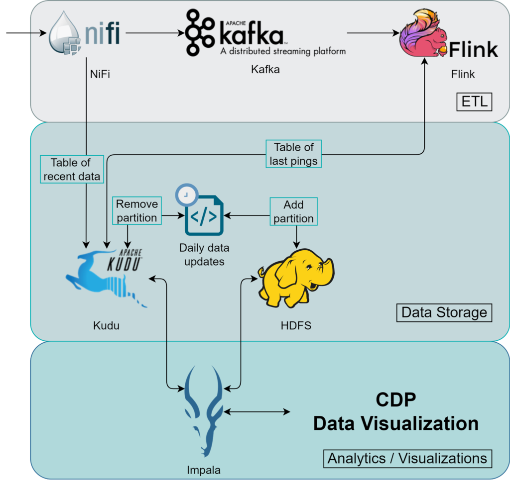
Image 1: Schema of the data pipeline for the IoT framework in CDP.

The IoT data is directed to NiFi’s HTTP endpoints (see our blog post on how to use NiFi to provide HTTP endpoints). NiFi, like all Cloudera tools, offers significant and straightforward scalability, so you can scale NiFi according to the throughput of your IoT traffic. Adding more nodes in NiFi will add more HTTP endpoints too (which you can balance with an external load balancer), ensuring efficient ingestion of all your incoming IoT data. Once the data is in NiFi, the first thing we do is parse it to make sure that it has the necessary format. In other words, we modify the data to fit our requirements before saving it to our storage system.

After that, there are two paths: one directly stores the data in the ‘recent data’ table, overseen by Kudu, while the other uses Flink to perform UPSERT tasks. After checking some conditions, it stores the filtered, new data rows in a separate Kudu table that logs the latest pings from each sensor.

Kafka is used because it acts as the data source for Flink, so we need to publish from NiFi to Kafka to enable Flink processing on the data.

Up to this point, everything is managed with stream processing, which is advantageous as we use this data to monitor recent events with minimal latency. However, we want the data to be useful for more than just a few days. Historical data should always be accessible, but Kudu is not the best choice for massive storage. We opted for HDFS to solve that issue, a default storage solution inside Cloudera´s Hadoop ecosystem oriented to store huge amounts of data – what we can call a data lake.

The only issue posed by adding HDFS for historical data is the need to consult two distinct sources, HDFS and Kudu, every time we wish to execute a query to determine where to search for the data.

We solved this issue by automating the Sliding Window Pattern for Impala proposed by Grant Henke (a Cloudera software engineer). The benefits of this awesome design are:

• Leveraging the best features of each storage: HDFS and Kudu.
• Transparent querying to both storages from a single table.
• Improved performance for data analysts due to a simplified model.
• Daily maintenance time is significantly reduced through automation.

Since Impala supports querying from Kudu and HDFS, the user will be querying the whole dataset without having to know where each row is stored.

So, our final solution consists of historical data being kept in HDFS and recent data being stored in Kudu, with both being queried seamlessly from Impala. The automation of the maintenance is performed by a script that is run once a day and transfers the data from 3 days ago to HDFS.

Based on what we’ve shared up to this point, you may have already guessed some elements of the implementation. Let´s check them out together!

Implementation Details

For the technically minded among you eager to delve into the details, we’ve explained the construction of each service below. However, it might be a good idea to briefly revisit the use case we discussed in our previous blog post before diving deeper into the specifics.

The data we were exploring was about a city´s weather, air pollution levels, and water quality. From the point of view of the analytical platform, we are receiving HTTP requests comprising JSON files of measurements from sensors distributed around the city. These files provide insights into the sensor station sending the data – details like station id, coordinates, and location. Additionally, they include information about the individual sensors within that station – their sensor id, the kind of data they record, the specific measurement value, units, and so on.

We will stick to this use case in this second blog post too.

NiFi

The data flow in NiFi is, basically, what we explained when talking about the architecture.

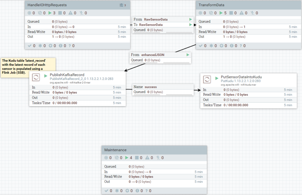
Image 2: Dataflow for the IoT framework implemented in NiFi.

First, NiFi handles the incoming HTTP requests (using HandleHTTPRequest) that contain the incoming data from the devices (assuming the devices send the data to HTTP endpoints as HTTP requests). Then it formats the data to what the downstream services require. In this IoT demonstration use case with weather data from stations in a city, the input data that arrives in NiFi is a JSON representing a whole station, so one thing we have to do in this transformation phase is to separate the measurements from each sensor within the station, allowing us to handle each measurement individually.

After that, we publish the data to Kafka and store it in Kudu as well. Note that there is another part being handled with Flink, but this is outside the scope of NiFi.

There’s also a maintenance task to automate the transition of data every 24 hours from recent to historical, i.e., from Kudu to HDFS.

Flink

After publishing to Kafka, we can use SQL Stream Builder (SSB) to perform SQL jobs in Flink, instead of having to write Java code. For example, we are running the following SQL code:

select src.sensor_id, src.station_id, cast(src.cust_timestamp as timestamp(3)) as cust_timestamp
from (
	select sensor_id, station_id, cast(cast(cust_timestamp as bigint)/1000 as timestamp) as cust_timestamp
	from `iot_data`
) src
left join `Kudu`.`default_database`.`impala::alex_db.latest_record` dst
	on src.`sensor_id` = dst.`sensor_id`
where src.cust_timestamp > dst.cust_timestamp

We have directed Flink to use the table

`Kudu`.`default_database`.`impala::alex_db.latest_record`

as the sink table:

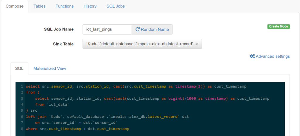
Image 3: : SSB’s UI with the specified sink table and the query.

We are using Flink to sift through the new rows of sensor data that are published to Kafka, keeping only the most recent entries in a separate Kudu table. This facilitates the effortless monitoring of the health of each station, and the filtering is necessary to avoid potential lags in inputs due to out-of-sequence deliveries.

Kudu

We chose Kudu to store the most recent data, plus an extra table that contains the most recent record for each sensor. Kudu is excellent for this use case because, with this constraint, there isn´t a huge amount of data and there´s also the table for the recent records, which is always changing. From this database, we will get the fastest queries with minimal latency.

The main table in Kudu is “iot_data_recent”, intended for storing the data from the last few days. In our use case, we chose to house the last 2 days in Kudu; the syntax to create it from Impala looks like this:

CREATE TABLE alex_db.iot_data_recent (
  sensor_id INT,
  cust_timestamp TIMESTAMP,
  station_id INT,
  lat DECIMAL(9, 6),
  long DECIMAL(9, 6),
  value DECIMAL(9, 4),
  units STRING,
  type STRING,
  location_name STRING,
  PRIMARY KEY (sensor_id, cust_timestamp)
) PARTITION BY HASH (sensor_id) PARTITIONS 3, 
RANGE (cust_timestamp)
(
  PARTITION '2023-01-19' <= VALUES < '2023-01-20',
  PARTITION '2023-01-20' <= VALUES < '2023-01-21'
)
STORED AS KUDU;

We use a hash partition based on sensor_id to leverage distributed storage and compute by evenly distributing the data across nodes. However, the real boost in performance for maintenance tasks comes from using range partitions with the dates: each range represents the data of a single day. Organising the data like this makes it easier to move a whole day’s data to HDFS, done daily; we’ll delve into the specifics of this process later.

There is a second table that we mentioned, used to keep track of the last time each sensor sent data. This is a simple table that does not even need to be partitioned – unless you intend to have hundreds of thousands of sensors, which is rarely the case.

HDFS

This table is the equivalent of the main Kudu table above, but it acts as the historical data storage. We can interact with it from Impala too. The syntax we used to create it is:

CREATE TABLE alex_db.iot_data_hist (
  sensor_id INT, 
  cust_timestamp TIMESTAMP, 
  station_id INT, 
  lat DECIMAL(9, 6), 
  long DECIMAL(9, 6), 
  value DECIMAL(9, 4), 
  units STRING, 
  type STRING, 
  location_name STRING, 
  PRIMARY KEY (sensor_id, cust_timestamp)
) PARTITIONED BY (cust_date DATE)
STORED AS PARQUET
TBLPROPERTIES (
  'transactional' = 'true',
  'transactional_properties' = 'insert_only'
);

Note that this table is partitioned by specific dates, instead of the range timestamps used in Kudu. When we get round to the unified view, we’ll demonstrate how to query transparently using a timestamp filter, even when there’s a date-type partition in HDFS.

View on Impala

Thanks to Impala´s ability to query Kudu and HDFS, we can unify the data in a view that merges both tables. What’s more, we can keep using a timestamp to filter the data when querying the view and the field will be automatically converted to a date to leverage partition pruning on HDFS. This process is invisible to the user, harnessing the strengths of both storage systems without complicating the model for the data analyst.

To see how we can get this feature, let’s imagine that today is January 20^th, 2023. We would have data from January 19 and 20 in Kudu, and older data in HDFS:

CREATE VIEW alex_db.iot_data AS 
SELECT 
  sensor_id, 
  cust_timestamp, 
  station_id, 
  lat, 
  `long`, 
  value, 
  units, 
  type, 
  location_name 
FROM 
  alex_db.iot_data_recent
WHERE 
  cust_timestamp >= '2023-01-19' 
UNION ALL 
SELECT 
  sensor_id, 
  cust_timestamp, 
  station_id, 
  lat, 
  `long`, 
  value, 
  units, 
  type, 
  location_name 
FROM 
  alex_db.iot_data_hist 
WHERE
  cust_date = CAST(cust_timestamp AS DATE)

The last WHERE clause converts the timestamp into a date format, which, thanks to partitioning, enhances HDFS’s efficiency. Kudu already uses the timestamp data type, so there’s no need for any additional modifications.

If we check the planning of the following query:

explain
select sensor_id
from iot_data
where cust_timestamp > '2022-01-20'

We can see that the path to complete it is:

Explain String
Max Per-Host Resource Reservation: Memory=256.00KB Threads=3
Per-Host Resource Estimates: Memory=52MB
PLAN-ROOT SINK
|
03:EXCHANGE [UNPARTITIONED]
|
00:UNION
| row-size=102B cardinality=564.49K
|
|--02:SCAN HDFS [alex_db.iot_data_hist]
| partition predicates: cust_date > DATE '2022-01-20'
| HDFS partitions=366/687 files=366 size=79.69KB
| predicates: alex_db.iot_data_hist.cust_timestamp > TIMESTAMP '2022-01-20 00:00:00', cust_date = CAST(cust_timestamp AS DATE)
| row-size=114B cardinality=560.02K
|
01:SCAN KUDU [alex_db.iot_data_recent]
kudu predicates: alex_db.iot_data_recent.cust_timestamp > TIMESTAMP '2022-01-20 00:00:00', cust_timestamp >= TIMESTAMP '2023-01-19 00:00:00'
row-size=114B cardinality=4.47K

We are querying from both sources because we are targeting everything after ‘2022-01-20’. We can also see that only 366 HDFS partitions are being used, from the 687 we have, because we do not need to check for rows in older partitions.

Another example of how this works is to query specific data stored only in Kudu:

explain
select sensor_id
from iot_data
where cust_timestamp > '2023-01-19'

With the previous query, we see this result:

Explain String
Max Per-Host Resource Reservation: Memory=0B Threads=2
Per-Host Resource Estimates: Memory=10MB
Codegen disabled by planner
PLAN-ROOT SINK
|
00:UNION
| row-size=4B cardinality=2.24K
|
|--02:SCAN HDFS [alex_db.iot_data_hist]
| partition predicates: mydate > DATE '2023-01-19'
| partitions=0/31 files=0 size=0B
| predicates: alex_db.iot_data_hist_.cust_timestamp > TIMESTAMP '2023-01-19 00:00:00', cust_date = CAST(cust_timestamp AS DATE)
| row-size=24B cardinality=0
|
01:SCAN KUDU [alex_db.iot_data_recent]
kudu predicates: alex_db.iot_data_recent.cust_timestamp > TIMESTAMP '2023-01-19 00:00:00', cust_timestamp >= TIMESTAMP '2023-01-19 00:00:00'
row-size=4B cardinality=2.24K

Only Kudu contains the data we are querying. We can see that no partition is read on HDFS due to the date-based partitioning.

Scripts For Maintenance

For perfect scalability with upcoming dates, we can automate moving the data from Kudu to HDFS and create new date partitions.

We achieved this by scheduling the execution of bash scripts that use the “impala-shell” command to run queries such as:

INSERT INTO alex_db.${var:hdfs_table} PARTITION (cust_date)
SELECT *, cast(cust_timestamp as DATE)
FROM alex_db.${var:kudu_table}
WHERE cust_timestamp >= "${var:new_boundary_time}"
AND cust_timestamp < days_add("${var:new_boundary_time}", 1);

COMPUTE INCREMENTAL STATS alex_db.${var:hdfs_table};

This query moves the data from Kudu to HDFS and computes the stats incrementally. Please note that the syntax accepts variables that can be specified in the command´s input arguments. You can check out Grant Henke´s blog post (which we mentioned above) to get an in-depth view of how this works.

Visualisations

We´ve reached the last stage of the data cycle, where we can really see its true value!

As we mentioned in the first part of this series, there are endless ways we could analyse our data, but we are only going to focus on a few examples of visualisation to keep things simple.

The tool we are using is Cloudera Data Visualization, just to stay in the Cloudera environment, but any other BI tool could be used.

In Cloudera Data Visualization, we are going to use the table from Impala to query the main tables in Kudu and HDFS transparently.

The following image shows an example of what we can get from this implementation:

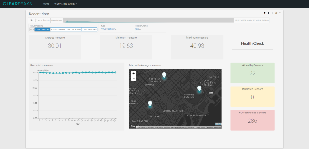
Image 4: One of the tabs from the dashboard developed for the demo, with dummy data

As you can see, it shows us average, minimum, and maximum temperatures, together with an interactive map of the location of the station, and it also tracks the number of sensors that sent the data correctly on time.

In this example we are applying a filter for the last 10 hours, but we could also make it wider and include data from the last month. We would only have to target the view on Impala that joins historical and recent data, then the filters on partitions would route the query to the correct storage.

This would not be a problem for our sensor Health Check, because these up-to-date records are stored on a separate table in Kudu.

Conclusions

We hope you’ve enjoyed reading our two-part mini-series on our IoT framework! In the first blog post we introduced a data generator to simulate a realistic stream of IoT data, and in this second part we’ve seen how IoT data, be it simulated or real, can be ingested, analysed and visualised.

Our framework offers a unique solution that ensures your data retains its value over time and enables real-time monitoring with IoT sensors. It’s also easily and cost-effectively scalable due to the nature of Cloudera services.

We’ve also demonstrated the use of Impala, HDFS and Kudu to extract value from the data and to run a simple health check on the sensors, showcasing how these tools can be leveraged to store historical data in an append-only manner while simultaneously providing real-time insights thanks to NiFi and Flink.

Although we based our mini-series on a specific environmental data use case, remember that our framework can be extended to other industries as well. If your business needs to monitor any device, machine or even an agricultural plantation, this would be the perfect approach.

Future Steps

Like everything in the world of software, this is an evolving tool that will grow with more features as we detect new challenges.

A logical next step could be the integration of an orchestration tool to further automate our solution to help with faster decisions in response to changes in patterns or errors in the data.

If you have any questions or comments about our IoT framework or would like to learn more about our solutions and services, please don’t hesitate to contact us. Our team of certified experts will be happy to help you make informed decisions about your projects.