16 Nov 2022 Massive Survey Data Exploration with Dremio (Part 1)

As the amount of data piles up it is crucial to be able to manage that growth and not let our tools fall behind; we must analyse the use case and choose a suitable platform to handle the data as it grows.

This is the first of a two-part series where we are going to discuss a use case related to a massive survey dataset, scaling up to 1 billion rows of data, on which we have been working recently for one of our customers. The dataset contains the answers to multiple surveys, each survey having hundreds of questions and being answered by tens of thousands of people.

Initially, due to the volume of data, our customer was only loading a few surveys into a RDBMS, and some reports were created with a BI tool to enable analysis. To achieve fast responses, our customer leveraged extracts provided by the BI tool. This solution was working well enough for a low number of surveys (with tens of millions of rows), but our customer was worried about the cost of analysing the data from more surveys whilst maintaining reasonable query response times. The goal was to get responses within 10 seconds to most of the ad hoc queries and the BI tool visualisations.

As the data would grow (with more surveys being added), the extracts of the BI tool would also grow and the cost (BI tool licence and hardware, but especially the licence) would also grow significantly – our customer calculated what the cost would be when dealing with a billion rows, and it was plainly unreasonable.

And that is when we came in – what we proposed to handle this amount of information was to change the storage to a data lake and to use a powerful and scalable query engine able to work directly on the data lake. This would move the workload from the BI tool extracts to the query engine, and the storage to the data lake, thus reducing costs. The perfect fit was Dremio, which thanks to its reflections (its flagship feature), enables running fast SQL queries from the data stored in the AWS S3 data lake. Note that the solution would also work on other cloud storage or data lake technologies; another benefit of our solution is that it works with pretty much any BI tool. Since Dremio offers outstanding compatibility with Power BI – one of our favourites – we have, for the sake of these blogs, reproduced some of the customer dashboards in Power BI.

In this article we are going to see how we can accelerate queries with Dremio in this real use case with massive survey data. We are going to run through a brief introduction to Dremio reflections and how we used them to improve the performance of some plain SQL queries executed on this massive dataset. In the next part of this series, we will focus on accelerating the queries from the BI tool visualisations, i.e., Power BI, which may use different filters in each execution.

Before going into more detail, we recommend reading our previous blog post about Dremio for an introduction to this fantastic data lakehouse platform, to understand how it achieves query acceleration via reflections, and to see how it can be deployed on a cloud such as AWS. And if you’re short on time, there’s a brief introduction to Dremio in this blog post too!

1. Introducing Dremio

Dremio is a data lakehouse SQL engine that excels at dealing with large amounts of data from multiple sources simultaneously at an end-user level (BI, analytics, etc.), as well as working directly with data lakes.

The way Dremio improves performance is by using reflections – these are physically optimised representations of the source data. Reflections can be raw or aggregated. In all cases they use optimal file and table formats (under-the-hood optimisations such as those provided by Iceberg are used, as are partitioning and sorting). The main difference between the two types is that raw reflections are useful for focusing on a subset of the data or simply enhancing its format, whereas aggregation reflections are more suitable when the data is going to be queried in a BI fashion (i.e., using “GROUP BY” statements), because essentially Dremio stores precomputed aggregations based on the fields defined in the reflection definition.

Another important thing to bear in mind is that Dremio uses “elastic engines”, which in the case of AWS, are EC2 instances; these are the worker nodes of the architecture that will handle the workloads.

For this project we are using a single elastic engine with m5d.2xlarge EC2 nodes: 1 coordinator and 4 workers. However, we can set Dremio to use more engines and to automatically upscale or downscale in response to the workload and the number of users (for example, there could be sets of users using dedicated engines, so they have isolated computing resources).

Now that we have seen how Dremio works, let’s move on to the dataset.

2. The Dataset

We have the following dataset of 1 billion rows, which contains the fact table “V_SURVEY_FEEDBACK” and 17 other dimensions:

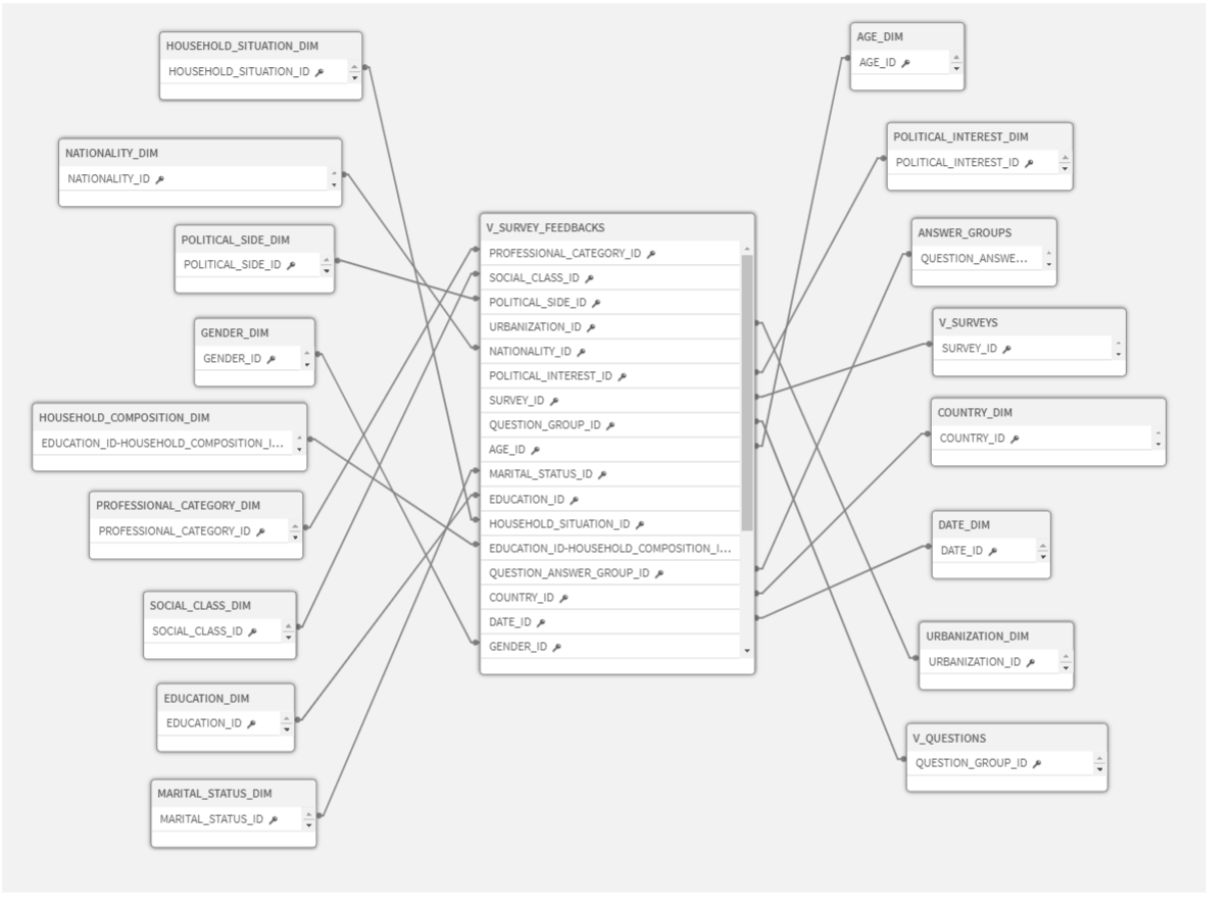
Figure 1: Massive survey dataset

Each time a user completes a survey, the results are stored in S3. Since it is a data lake, it is designed to handle enormous amounts of data, so we can store anything we want without worrying about capacity.

Please note that the data used and shown in these blog posts is synthetic data and does not correspond to any existing survey.

2.1. Adding the Physical Dataset

Once we know which dataset we are dealing with, we can start setting everything up to enable Dremio to query the data.

First, we need to add a connection to “S3 Data Lake” by giving the access key and access secret of the account that has access to the bucket:

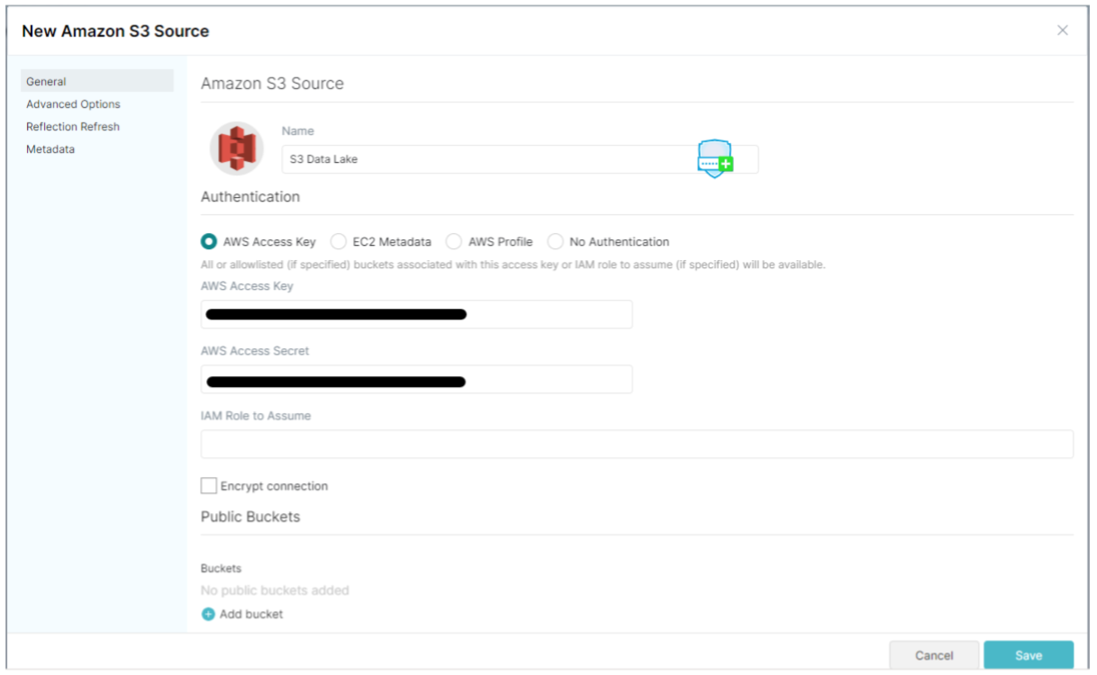
Figure 2: Menu to add a new S3 source

Now we can start specifying the datasets we want to use from our S3 storage by clicking on “S3 Data Lake”, in the lower-left corner:

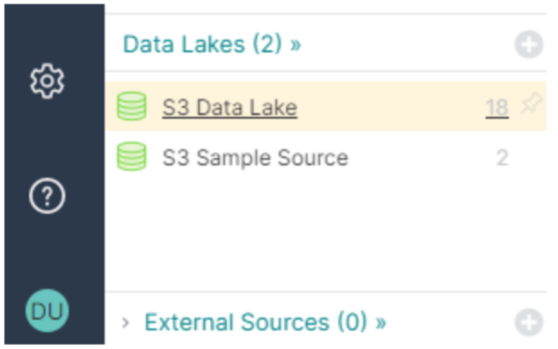
Figure 3: Button to access the S3 data

This opens a browser where we can get to the actual object we want to use as the source. We can select a whole folder for a single table, as is the case for the fact table, by hovering the mouse over an object and selecting the button that appears on the right:

Figure 4: Button to convert a folder into a source dataset

Once we have selected an object as the source, a window pops up, where we specify the format of the data to allow Dremio to read it properly:

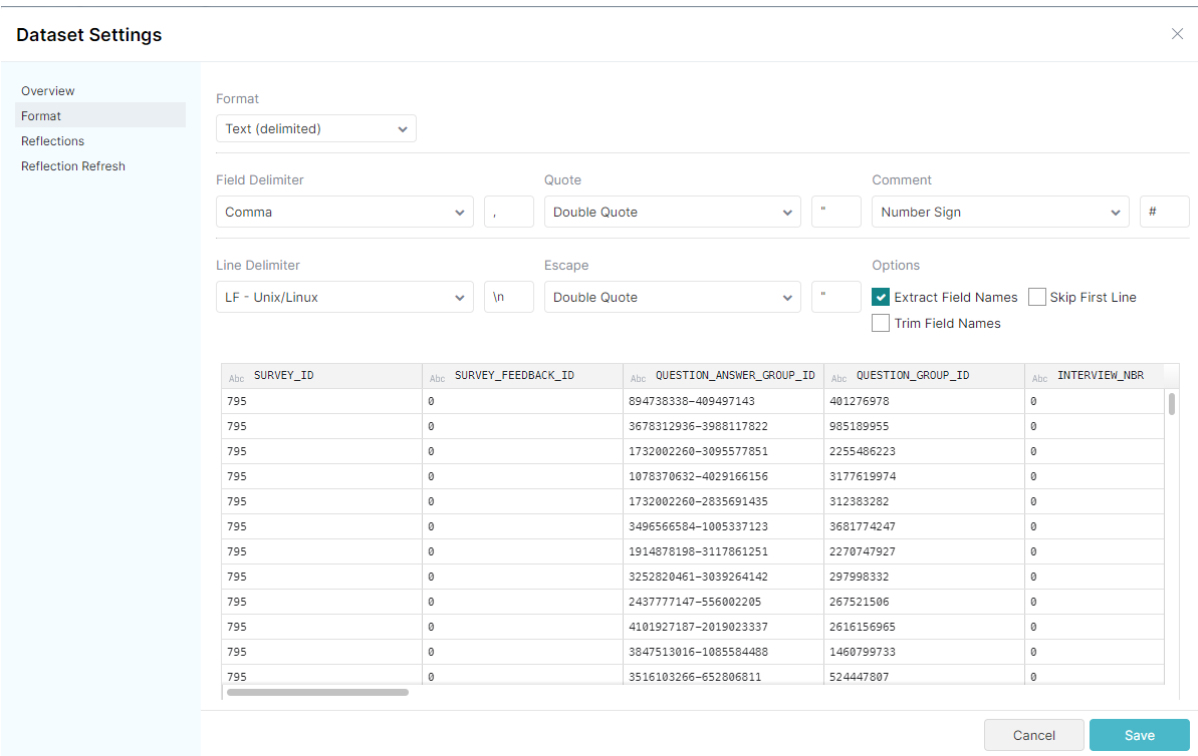
Figure 5: Dataset format window

For the rest of the tables, we’ll select each individual object as they only have one file per table:

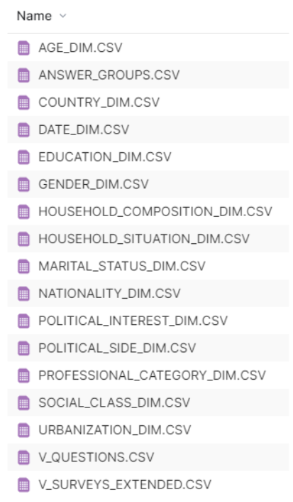
Figure 6: List of datasets for the dimension tables

Remember that Dremio does not load the data, and the S3 objects we have selected will remain in the same place; we’ve only told Dremio how to read the data in S3.

Now that all the sources are set up, we can start with the views.

3. Views

We can create views on top of the physical datasets. A view is a virtual table, created by running SQL statements or functions on a physical table or another view.

It is recommended that the views are made incrementally, creating multiple layers of views.

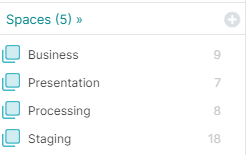
Figure 7: Different layers that a Dremio project may contain

The first layer is Staging: here we will be performing 1-1 views from the physical tables we previously added from S3, so each physical table will have a view created of it. We’ll also correct the names of the columns, their type, and make any additional changes, such as calculated fields, if necessary.

One example of a change we need to perform is to separate the field “question_answer_group_id” into two different ones: “question_id” and “answer_group_id”. To separate these two fields, we can go to the virtual “survey_feedback” table and click on the dropdown menu of the problematic field:

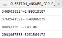
Figure 8: Preview of the QUESTION_ANSWER_GROUP_ID column, inside the survey_feedback table

We then select ‘Extract Text…’ to select the left side of the field, and then the right side (e.g.: ‘12345-54321’ becomes ‘12345’ and ‘54321’):

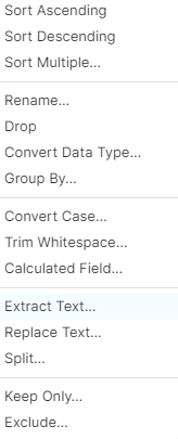
Figure 9: Dropdown menu for a single column

We extract by pattern, from the “First” match, with the regular expression “\d+” to select a number with multiple digits. Be careful not to check the ‘Drop Source Field’ option, as we need to maintain the source field for joins:

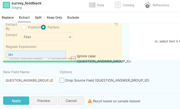
Figure 10: Extract Text menu

We’ll name the resulting field “question_id”. Afterwards, we repeat the same actions but select the “Last” match instead, and name the resulting field “answer_group_id”.

Finally, we want to make sure that our data is in an optimised format, so if it is not already stored in Apache Parquet (or similar) we should make a raw reflection of the 1-1 view.

For the following layers of views, we will be focusing more on the queries we want to cover.

So far we have seen how to add physical datasets to Dremio, how to adapt the data with 1-1 views, and we have also ensured that the data is in an optimised format. We’re all set to start with more reflections, but first let’s take a look at the queries we want to accelerate to plan the next steps properly.

4. Queries

The goal of the data is to meet business needs which, in this case, are visual reports that offer key insights. These visualisations made with our BI tool (Power BI) create queries that are passed to Dremio, where they are executed to retrieve the data from S3.

In addition to these queries from the visualisation itself, we also have some extra queries to help understand how reflections work and how to improve performance. In our next blog post we’ll cover a more realistic use case with Power BI.

4.1. Example Query

Take a look at the following query:

-- Percentage of participants grouped by age range filtered per year 
with groupNA as ( 
    select "year", 
    count(survey_id) total_filt_answers 
    from Processing.sf_a_d 
    where age_id >= 100 or age_id = 5 or age_id = 0 
            and "year" > 2018 
    group by "year" 
), 
group15_24 as ( 
    select "year", 
    count(survey_id) total_filt_answers 
    from Processing.sf_a_d 
    where age_id >= 15 and age_id < 25 or age_id = 1 
            and "year" > 2018 
    group by "year" 
), 
group25_39 as ( 
    select "year", 
    count(survey_id) total_filt_answers 
    from Processing.sf_a_d 
    where age_id >= 25 and age_id < 40 or age_id = 2 
            and "year" > 2018 
    group by "year" 
), 
group40_54 as ( 
    select "year", 
    count(survey_id) total_filt_answers 
    from Processing.sf_a_d 
    where age_id >= 40 and age_id < 55 or age_id = 3 
            and "year" > 2018 
    group by "year" 
), 
group55_plus as ( 
    select "year", 
    count(survey_id) total_filt_answers 
    from Processing.sf_a_d 
    where age_id >= 55 and age_id < 100 or age_id = 4 
            and "year" > 2018 
    group by "year" 
), 
total_participants as ( 
    select count(survey_id) total_answers, "year" 
    from Processing.sf_a_d 
    group by "year" 
) 
select tot."year", 
    g15_24.total_filt_answers g15_24, 
    g25_39.total_filt_answers g25_39, 
    g40_54.total_filt_answers g40_54, 
    g55_plus.total_filt_answers g55_plus, 
    gna.total_filt_answers gna, 
    tot.total_answers 
from groupNA gna 
inner join group15_24 g15_24 on gna."year" = g15_24."year" 
inner join group25_39 g25_39 on gna."year" = g25_39."year" 
inner join group40_54 g40_54 on gna."year" = g40_54."year" 
inner join group55_plus g55_plus on gna."year" = g55_plus."year" 
inner join total_participants tot on gna."year" = tot."year" 
order by tot."year" desc 
; 

We simply count the number of surveys answered, grouped by year and filtered by age; then we select the total to be able to compare participation proportionally within each age range.

Note that the tables used in the query are joins of the S3 source data. The table Processing.sf_a_d means that the view is in the Processing layer and the joined tables are survey_feedback, answer_groups, and date_dim. We created this join to make it easier for the query planner to identify the view that contains the reflection for the query. In addition, to keep everything nice and tidy, we created the Processing layer for all the joins we need.

If we were to plot this query it would look something like this:

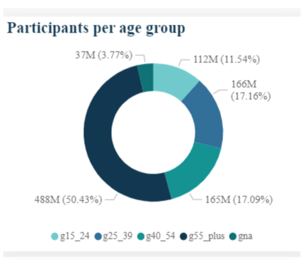
Figure 11: Plot of the percentage of participants grouped by age and filtered by yea

If we look closely at the query we can see a pattern; we only need to focus on one of the subqueries:

select "year", 
count(survey_id) total_filt_answers 
from Processing.sf_a_d 
where age_id >= 25 and age_id < 40 or age_id = 2 
             and "year" > 2018 
group by "year" 

Once we have managed to accelerate this one, all the others will be accelerated too (because they are identical, but with different values). There are no more aggregations outside the subqueries.

4.2. Reflection

The key to generating reflections is to create views that select the fields that participate in the query we want to accelerate, then build the reflection on top of this view.

Going back to the previous query, we wanted to focus on the subquery that appears multiple times. Creating the view for that is as simple as this:

select d."year", sf.survey_id, age.age_id 
from Staging.survey_feedback sf 
inner join Staging.age_dim age on sf.age_id = age.age_id 
inner join Staging.date_dim d on sf.date_id = d.date_id 

The reflection for that view would be an aggregate reflection with:

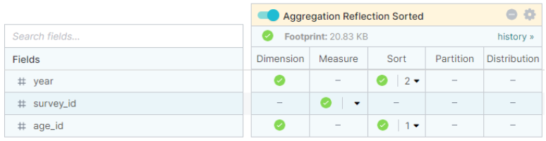
Figure 12: Reflection to accelerate the query of the percentage of participants grouped by age and filtered by year

After creating the reflection, we execute the query to test its performance:

Figure 13: Execution details for the percentage of participants grouped by age and filtered by year query

We can see an impressive execution time of 2 seconds for 1B rows!

4.3. More Queries

Here’s another query for the same dataset:

-- Gender difference on top 5 answered surveys by de predominant gender 
with total_participation as ( 
    select survey_id, count(survey_id) n_answers 
    from Processing.sf_g 
    group by survey_id 
), 
man_participation as ( 
    select survey_id, count(survey_id) n_answers 
    from Processing.sf_g 
    where gender_id = 1 
    group by survey_id 
), 
woman_participation as ( 
    select survey_id, count(survey_id) n_answers 
    from Processing.sf_g 
    where gender_id = 2 
    group by survey_id 
) 
select m.survey_id, m.n_answers man_ans, w.n_answers woman_ans, 
    cast(m.n_answers as float)/(t.n_answers)*100 man_pct, 
    cast(w.n_answers as float)/(t.n_answers)*100 woman_pct, 
    ( 
        select max(max_gender) 
        from (values(m.n_answers), (w.n_answers)) as gender_max(max_gender) 
    ) as max_gender 
from man_participation m 
inner join woman_participation w on m.survey_id = w.survey_id 
inner join total_participation t on m.survey_id = t.survey_id 
order by cast(max_gender as float)/(t.n_answers) desc 
limit 5 
; 

One way we could represent this query with a chart would be:

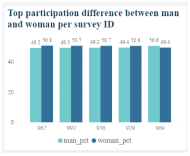
Figure 14: Representation of top gender difference in participation surve

Here’s another pattern-based approach – we count participation in each survey while filtering by gender:

select survey_id, count(survey_id) n_answers 
from Processing.sf_g 
where gender_id = 2 
group by survey_id 

In addition to this we also have another subquery with an aggregation that is unlike the other subqueries:

select max(max_gender) 
from (values(m.n_answers), (w.n_answers)) as gender_max(max_gender) 

The first thing is to create a view with all the participating fields; then we build the reflection selecting the following fields:

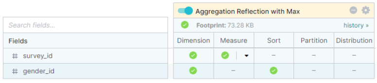
Figure 15: Reflection, with count and max as the measures, of the gender difference in answered surveys query

And the execution time for this query is:

Figure 16: Execution details of the gender difference in answered surveys query

We have one last query before going to the visualisation. This splits two queries that work together (one selects from the other):

-- Surveys that are more than 5% longer (on questions) than the average. 
with question_count as ( 
    select survey_id, count(distinct question_id) cnt_questions 
    from Staging.survey_feedback sf 
    group by survey_id 
), 
avg_questions_per_survey as ( 
    select ceil(avg(cnt_questions)) avg_q_per_survey 
    from question_count qc 
) 
select survey_id longer_survey, cnt_questions-(select avg_q_per_survey from 
avg_questions_per_survey) question_diff 
from question_count qc 
where cnt_questions > (select avg_q_per_survey from avg_questions_per_survey)*1.05 
; 

We need to focus on this subquery:

select survey_id, count(distinct question_id) cnt_questions 
from Staging.survey_feedback sf 
group by survey_id 

And the following subquery, which selects from the previous one:

select ceil(avg(cnt_questions)) avg_q_per_survey 
from question_count qc 

To accelerate this, we are going to create two views, and a reflection on top of each of them.

The first view is focused on the root subquery:

select survey_id, question_id 
from Staging.survey_feedback sf 

With the following reflection:

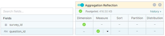
Figure 17: Reflection, with count as the measure, for the root subquery of the 5% larger surveys quer

And the second view is oriented to accelerate the next:

with question_count as( 
    select survey_id, count(distinct question_id) cnt_questions 
    from Staging.survey_feedback sf 
    group by survey_id 
) 
select cnt_questions 
from question_count

With the following reflection:

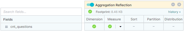
Figure 18: Reflection, with count and sum as the measures, for the outermost subquery of the 5% larger surveys query

Note that the second view we created stems from the root subquery, so that we can select the measures of the reflection based on the previous calculation.

Then we can execute the query and check that both reflections were used:

Figure 19: Job details on the reflections used for the execution of the 5% larger surveys query

And the execution time is:

Figure 20: Execution details of the 5% larger surveys query

Now that we have seen how we can create top-notch reflections for our queries, let’s run through the last topic in this article.

4.4. Incremental Reflections

Before creating reflections it is important to have the data ready to guarantee faster creation and the ability to carry out other types of queries.

In this case, we know that the data will always be queried by some specific fields, meaning that there will be restricting filters like:

WHERE question_id = ‘123456’

So a good foundation consists of creating a “general purpose” raw reflection on top of the fact table. This reflection will be partitioned by those fields used on restricted filters and those that appear in joins, although it is not advisable to use a lot of partitioning fields. We can build this reflection directly in the Staging layer.

We end up with a reflection like this:

Figure 21: General purpose reflection built on top of the virtualisation of the fact table

With this reflection, we see how the other reflections from the layers in Staging are created faster, and that all queries will be accelerated even if we don’t build another reflection oriented to the query in question.

Now that we have seen how we can leverage reflections to accelerate queries, we are ready to start with the second part, where we will focus on a more realistic use case: querying from the plots created with a BI tool like Power BI.

5. Next Steps

In our next blog post, we will see how to prepare reflections to accelerate BI-oriented queries that apply different filters for the same plot. We will also see how keeping reflections simple is sometimes better, with execution times to prove this!

If you have any questions about this blog post, Dremio, or building the most suitable architecture for your business, contact us and our certified experts will be happy to help you. Here at ClearPeaks we have ample experience in dealing with data no matter the field: Business Intelligence, Big Data, Machine Learning, and more!