24 Nov 2022 Massive Survey Data Exploration with Dremio (Part 2)

Welcome to the second and final instalment of our 2-part mini-series about how we used Dremio to analyse a massive survey dataset with over 1 billion rows for one of our customers. We recommend you check out the first blog post in this series, where we:

• Created the Staging layer, where we defined views and made the final changes to the data (such as splitting a column into two).
• Created “general purpose” raw reflections as well as aggregated reflections considering the queries we wanted to cover.
• Ran a set of plain SQL analysis queries in under 2 seconds thanks to the reflections created.

To quickly recap the use case, our customer had a lot of visualisations in a BI tool to analyse a survey dataset. They were leveraging the extracts managed by the BI tool to achieve fast responses. This solution worked fine for small datasets (a few million rows) but for bigger datasets (up to 1 billion rows) the hardware and licensing costs associated with the BI server would render it invalid.

We suggested our customer stopped relying exclusively on the BI tool and its extracts, and instead move the data to a data lake and the computing logic (equivalent to the extracts) to a powerful and scalable back-end SQL engine such as Dremio. This allows for a small front-end BI server, thus reducing costs significantly, whilst the storage is all in a data lake (much cheaper than storing data on extracts) and all the compute part is done (and governed, thanks to good semantic modelling in Dremio) in the back-end engine, offering an easier, scalable approach.

In the first blog post we saw how we could use reflections to minimise the response times of plain SQL queries; today we want to minimise the loading times of the visualisations of a BI tool, in this case Power BI. We have a Power BI dashboard that is equivalent to a subset of the visualisations the customer has in a different BI tool.

1.  Visualisations

When we create a BI dashboard, it is almost certain that we will be using lots of different filters. These filters add complexity to the queries (BI tools are going to fill our dashboards by creating queries that the back-end SQL engine, Dremio in our case, will execute). As we saw in the previous blog post, we can simplify the Dremio planning process by creating views (virtual tables) that join the data we are querying (a fact table and few dimension tables) and then by creating reflections on top of the views; and if we use aggregation reflections, we can get even faster responses. This approach works well when joining a low number of tables or dimensions, but creating aggregation reflections on top of views that join many tables or dimensions scales poorly when the number of dimensions to add to the reflections increases.

Imagine a measure that depends on 16 filters: we would have to create an aggregate reflection with 1 measure and 16 dimensions. Its creation would be time-consuming and it would also occupy a lot of space (although this would be the least of our worries when working with a data lake), because the measure in an aggregate reflection is calculated for all the combinations of dimensions. And remember that using a single aggregate reflection to cover lots of filters will cause your query to handle a huge workload in a single thread of tasks, so you will not be able to parallelise the query optimally and it will very likely run slower.

We can examine the execution plan of a query by going to the “Execution” tab inside the job details; this is useful for checking things like concurrency and runtime. Here is a sneak peek of what we see when checking the planning of a query:

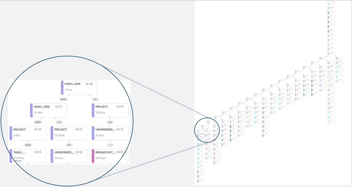
Figure 1: Execution plan of a query with multiple threads of tasks; accessible from the “Execution” tab of the job details

So, when we’ve got a fact table and some dimension tables and when we’re going to use views and reflections to feed our BI dashboard, the possibilities (including those we would discard) are shown below:

• Avoid creating views that join the data and don’t define the “join” at the BI tool. This might lead to very complex queries being thrown at Dremio, with Dremio unable to find the most suitable reflection for the executed queries.
• Create a view that joins the fact table with all 17 dimension tables to simplify the Dremio planner’s job, plus one of the following:
  • Create an aggregation reflection with all the filtering fields. This would cause slow queries due to the huge workload in a single aggregation reflection.
  • Create very small aggregation reflections with fewer filtering fields. This seems unreasonable because we would have to cover all the possible combinations of filters, which would waste a lot of time, and the Dremio planning part of a query would also take longer due to the numerous reflections it would have to consider.
  • Do not use aggregation reflections at all and rely on raw reflections. This isn’t a bad idea, but proper aggregation reflections can accelerate our queries much more.
  • Use aggregation reflections for queries with fewer dimensions and raw reflections for queries with more dimensions. This is the best approach we have found for our case.

We’ve already learned one important lesson: we can use the view of a join of tables to query and to build aggregation reflections with a small number of dimensions. However, when facing numerous dimensions (or high-cardinality dimensions), you can still use the view of the join but let the multiple raw reflections accelerate the query.

We will demonstrate this by showing the results of the following methodologies:

1.1. Connection to Dremio

There are many ways to connect Power BI to Dremio; we used the “Get data” button from the “Home” menu in PBI.

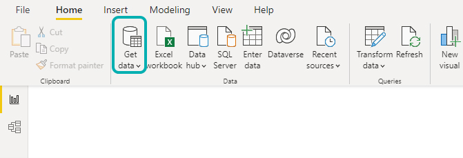
Figure 2: Connection to Dremio from Power BI

When the new window appears we can search for “Dremio” and select the version we are using, Dremio Software in our case:

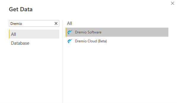
Figure 3: Selecting Dremio as the query engine for Power BI

Then we have to specify the server’s IP and the port to connect with Power BI, 31010. We also need to specify if there is any encryption (or not) and the connectivity mode, in our case “DirectQuery”, so that all the workload stays in Dremio (1 billion rows in import mode would be unrealistic due to the amount of time needed to load the data; this is one of the things we wanted to avoid from the start, by separating compute and storage).

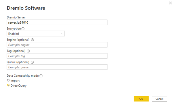
Figure 4: Configuring the connection to Dremio in Power BI

After clicking on “OK” a new window to log in to Dremio will appear. Enter the necessary credentials, and a new window with a navigator will appear where we can browse all the views and raw data in Dremio and select them as the data source for our plots:

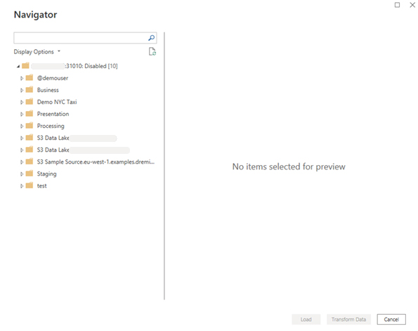
Figure 5: Navigator window, where we can browse our Dremio project

We can select as many of the tables as we want. Since we are showing the queries without a join first, we’ll select all the tables in the Staging layer:

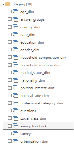
Figure 6: The virtual tables from the Staging layer

Now that all the fields have been loaded into the menu on the right, we are ready to create relationships between tables. We do this by clicking on the “Model” tab, on the left side of the screen:

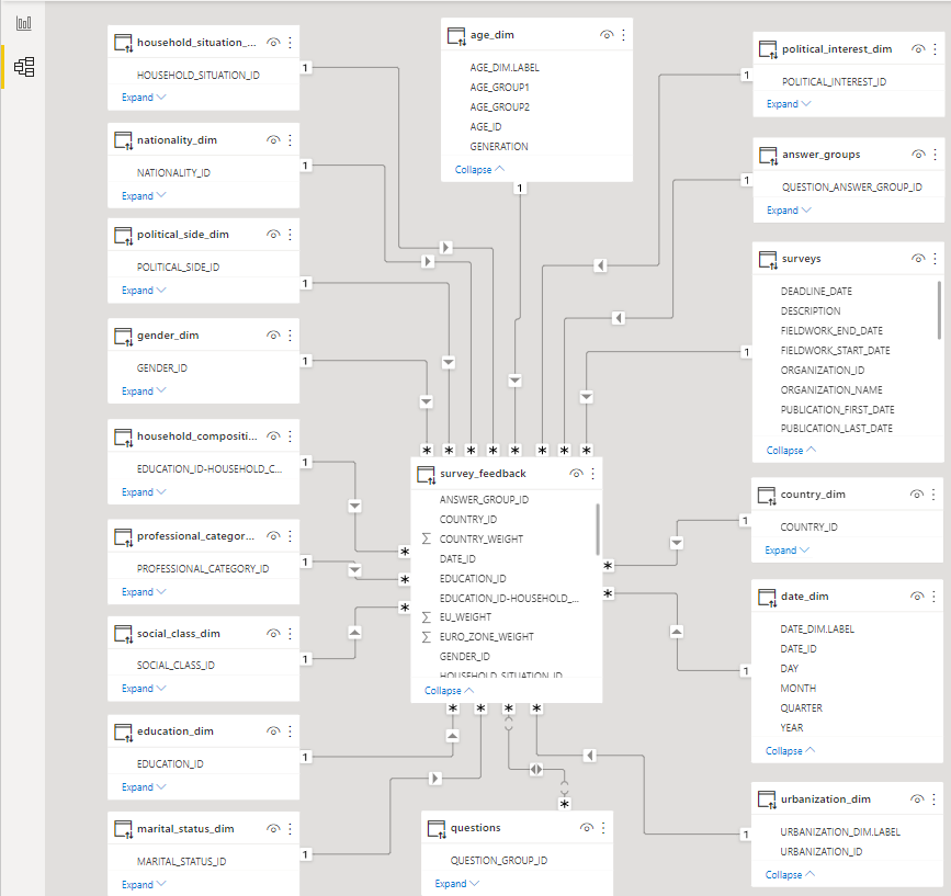
Figure 7: Data model in Power BI

Now everything is set up and we can start with the visualisations.

1.2. The Dashboard

We have a dashboard consisting of different visuals, each of them filtered by a mandatory filter (“question_id”); there are also some different optional filters around each chart. It looks like this:

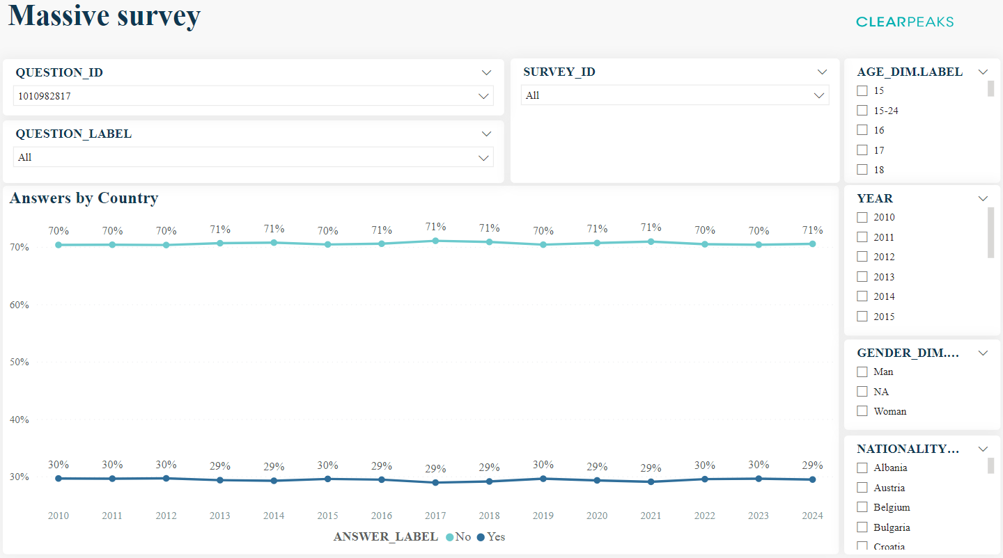
Figure 8: Example of a dashboard for the massive survey dataset

To simplify things, let’s just focus on the following visual where we can see the proportion of the different answers by country:

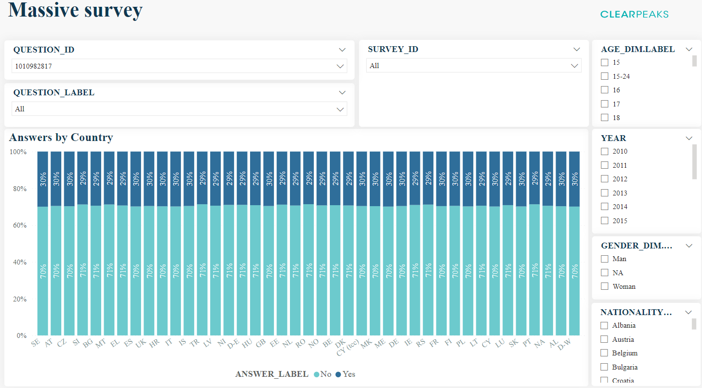
Figure 9: Answers by Country chart with the filters around it

First we’ll create the visual and then check the job that will have been produced in Dremio to fulfill the query needed by Power BI to complete the plot.

1.3. Plotting the Chart

Before starting on the chart, we’ll create a calculated field to help count all the answers:

# Answer % =  
var total  = calculate(COUNT(survey_feedback[SURVEY_ID]),  
ALL(answer_groups[ANSWER_LABEL])) 
var target = calculate(COUNT(survey_feedback[SURVEY_ID])) 
return divide(target, total, 0)

Then we use a stacked bar chart with the following fields:

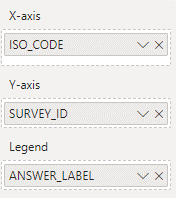
Figure 10: Selected fields to plot the visual in Power BI

We can see the mandatory filter, “question_id”, in the top-left corner of the dashboard:

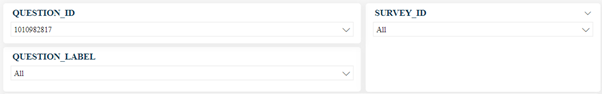
Figure 11: The mandatory filter “question_id” and other optional filters

There are some other optional fields on the right:

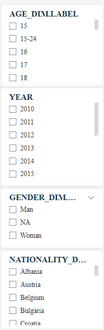
Figure 12: Filtering dimensions

The result of the chart is as follows:

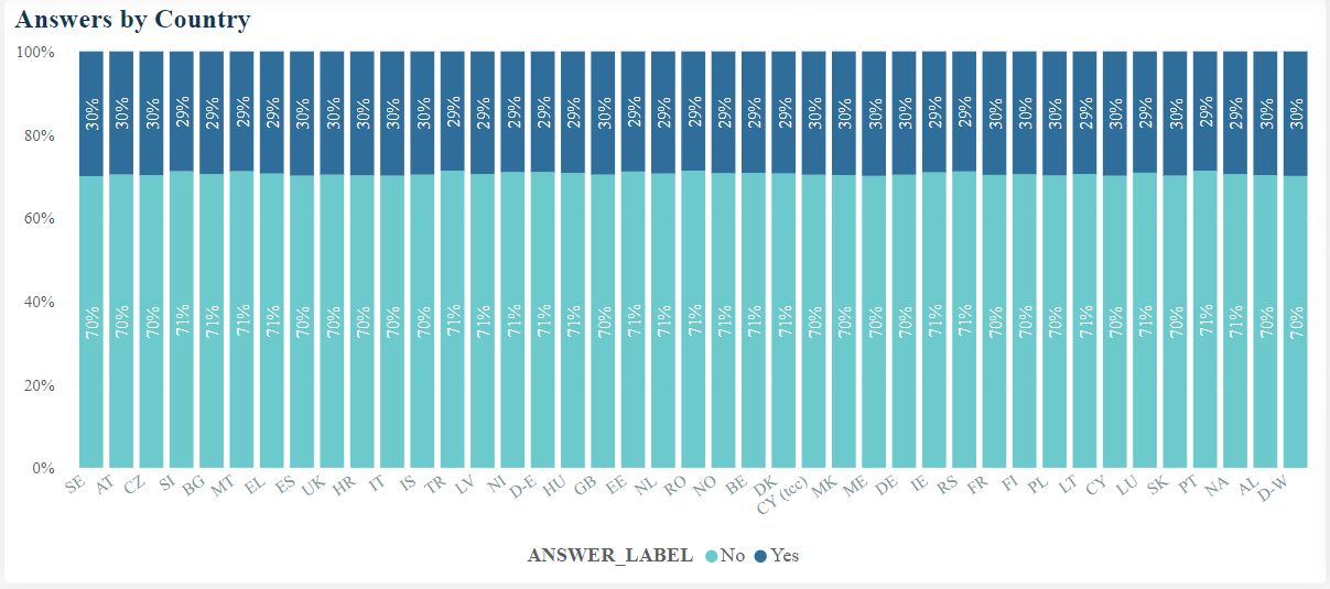
Figure 13: Chart of the proportion of answers by country; for the selected question_id, the only possible answers are “Yes” or “No”

1.4. Running the Dashboard

Once the chart has been created, Power BI creates the query that the query engine will execute. If we go to Dremio’s job history, we can see the job that has been processed:

Figure 14: Execution details of querying without a join or filters

It took 18 seconds to plot the previous chart; we can also check the exact query that was executed:

select `ANSWER_LABEL`,
    `ISO_CODE`,
    count(`SURVEY_ID`) as `C1`
from 
(
    select `OTBL`.`SURVEY_ID`,
        `OTBL`.`ANSWER_LABEL`,
        `ITBL`.`ISO_CODE`
    from 
    (
        select `OTBL`.`SURVEY_ID`,
            `OTBL`.`SURVEY_FEEDBACK_ID`,
            `OTBL`.`ANSWER_GROUP_ID`,
            `OTBL`.`QUESTION_ID`,
            ...
            `ITBL`.`ANSWER_GROUPS.LABEL`
        from `Staging`.`survey_feedback` as `OTBL`
        inner join 
        (
            select `ANSWER_CODE`,
                `QUESTION_ANSWER_GROUP_ID`,
                `ANSWER_GROUP_ID`,
                `QUESTION_ID`,
                `ANSWER_LABEL`,
                `ANSWER_GROUPS.LABEL`
            from `Staging`.`answer_groups`
            where `QUESTION_ID` = '1010982817'
        ) as `ITBL` on (`OTBL`.`QUESTION_ANSWER_GROUP_ID` = 
`ITBL`.`QUESTION_ANSWER_GROUP_ID`)
    ) as `OTBL`
    inner join `Staging`.`country_dim` as `ITBL` on 
(`OTBL`.`COUNTRY_ID` = `ITBL`.`COUNTRY_ID`)
) as `ITBL`
group by `ANSWER_LABEL`,
    `ISO_CODE`
OFFSET 0 ROWS FETCH FIRST 1000001 ROWS ONLY

We can observe a certain complexity with the subqueries and joins; we will see later on how this can be simplified using the join we mentioned before.

Now let’s see what happens when we apply more filters to the dashboard. For example, we can apply:

• Age range of 15-24.
• Only men.
• People of Austrian nationality.

The result for executing the same chart with these filters is:

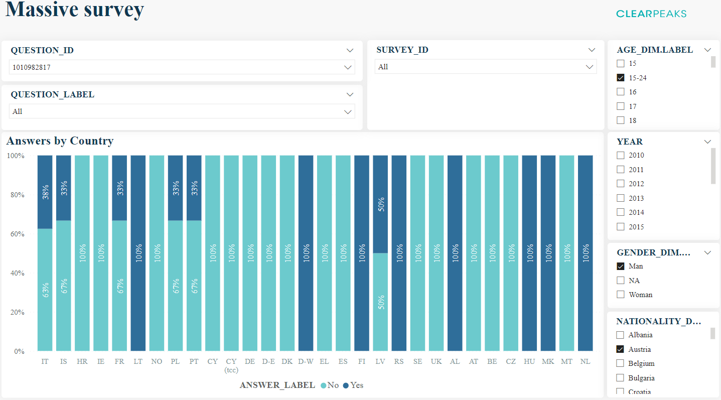
Figure 15: Answers by Country, filtered by an age range, a gender, and a nationality

And the details of the job processed in Dremio show a duration of 16 seconds:

Figure 16: Execution details of querying without a join and with filters

Taking a closer look at the query created by Power BI, we can see even more complex queries when adding filters (you don’t need to read it all, it’s just to highlight the complexity):

select `ANSWER_LABEL`,
    `ISO_CODE`,
    count(`SURVEY_ID`) as `C1`
from 
(
    select `OTBL`.`SURVEY_ID`,
        `OTBL`.`ANSWER_LABEL`,
        `OTBL`.`ISO_CODE`
    from 
    (
        select `OTBL`.`SURVEY_ID`,
            ...
            `ITBL`.`GENDER_DIM.LABEL`
        from 
        (
            select `OTBL`.`SURVEY_ID`,
                ...
                `ITBL`.`COUNTRY_DIM.COUNTRY_DIM.LABEL_GeoInfo`
            from 
            (
                select `OTBL`.`SURVEY_ID`,
                    ...
                    `ITBL`.`ANSWER_GROUPS.LABEL`
                from 
                (
                    select `OTBL`.`SURVEY_ID`,
                        ...
                        `ITBL`.`GENERATION`
                    from `Staging`.`survey_feedback` as `OTBL`
                    inner join 
                    (
                        select `AGE_ID`,
                            `AGE_DIM.LABEL`,
                            `AGE_GROUP1`,
                            `AGE_GROUP2`,
                            `GENERATION`
                        from `Staging`.`age_dim`
                        where `AGE_DIM.LABEL` = '40-54'
                    ) as `ITBL` on (`OTBL`.`AGE_ID` = `ITBL`.`AGE_ID`)
                ) as `OTBL`
                inner join 
                (
                    select `ANSWER_CODE`,
                        `QUESTION_ANSWER_GROUP_ID`,
                        `ANSWER_GROUP_ID`,
                        `QUESTION_ID`,
                        `ANSWER_LABEL`,
                        `ANSWER_GROUPS.LABEL`
                    from `Staging`.`answer_groups`
                    where `QUESTION_ID` = '1010982817'
                ) as `ITBL` on (`OTBL`.`QUESTION_ANSWER_GROUP_ID` = 
`ITBL`.`QUESTION_ANSWER_GROUP_ID`)
            ) as `OTBL`
            inner join `Staging`.`country_dim` as `ITBL` on (`OTBL`.`COUNTRY_ID` = 
`ITBL`.`COUNTRY_ID`)
        ) as `OTBL`
        inner join 
        (
            select `GENDER_ID`,
                `GENDER_DIM.LABEL`
            from `Staging`.`gender_dim`
            where `GENDER_DIM.LABEL` = 'Woman'
        ) as `ITBL` on (`OTBL`.`GENDER_ID` = `ITBL`.`GENDER_ID`)
    ) as `OTBL`
    inner join 
    (
        select `NATIONALITY_ID`,
            `NATIONALITY_DIM.LABEL`,
            `NATIONALITY_DIM.NATIONALITY_DIM.LABEL_GeoInfo`
        from `Staging`.`nationality_dim`
        where `NATIONALITY_DIM.LABEL` = 'Austria'
    ) as `ITBL` on (`OTBL`.`NATIONALITY_ID` = `ITBL`.`NATIONALITY_ID`)
) as `ITBL`
group by `ANSWER_LABEL`,
    `ISO_CODE`
OFFSET 0 ROWS FETCH FIRST 1000001 ROWS ONLY

We can reduce the complexity of the queries generated by the BI tool, and in the following sections we’ll go through joining the data before querying.

1.5. Joining the Data

Our approach is to create a new view that joins all the tables:

select *
from Staging.survey_feedback sf
inner join Staging.age_dim a on sf.AGE_ID = a.AGE_ID
inner join Staging.answer_groups ag on  sf.question_answer_group_id = 
ag.question_answer_group_id
inner join Staging.country_dim c on sf.country_id = c.country_id
inner join Staging.date_dim d on sf.date_id = d.date_id
inner join Staging.education_dim e on sf.education_id = e.education_id
inner join Staging.gender_dim g on sf.gender_id = g.gender_id
inner join Staging.household_composition_dim hc on sf.
"education_id-household_composition_id" = 
hc."education_id-household_composition_id"
inner join Staging.household_situation_dim hs on sf.household_situation_id = 
hs.household_situation_id
inner join Staging.marital_status_dim m on sf.marital_status_id = 
m.marital_status_id
inner join Staging.nationality_dim n on sf.nationality_id = n.nationality_id
inner join Staging.political_interest_dim pi on sf.political_interest_id = 
pi.political_interest_id
inner join Staging.political_side_dim ps on sf.political_side_id = 
ps.political_side_id
inner join Staging.professional_category_dim pc on sf.professional_category_id = 
pc.professional_category_id
inner join Staging.questions q on sf.question_group_id = q.question_group_id
inner join Staging.social_class_dim sc on sf.social_class_id = sc.social_class_id
inner join Staging.surveys s on sf.survey_id = s.survey_id
inner join Staging.urbanization_dim u on sf.urbanization_id = u.urbanization_id

We will plot everything from Power BI using this table; we don’t need to build the data model now because we are only using one table.

1.6. Optimising the Queries

After finishing the configuration of the dashboard again (changing the fields to use the ones from the join), we can check the job created in Dremio for this plot.

The query executed for the chart using only the “question_id” filter is shown below:

select `ANSWER_LABEL`,
    `ISO_CODE`,
    count(`SURVEY_ID`) as `C1`
from 
(
    select `SURVEY_ID`,
        `SURVEY_FEEDBACK_ID`,
        `ANSWER_GROUP_ID`,
        `QUESTION_ID`,
        ...
        `URBANIZATION_DIM.LABEL`
    from `Processing`.`all_join`
    where `QUESTION_ID` = '1010982817'
) as `ITBL`
group by `ANSWER_LABEL`,
    `ISO_CODE`
OFFSET 0 ROWS FETCH FIRST 1000001 ROWS ONLY

This query is much simpler than the one created without the join. To accelerate this query we can focus on the subquery that filters the table by “question_id” and groups by the dimensions “answer_label” and “iso_code”; there is also a count on “survey_id” over the previous dimensions.

A reflection we can use with this query is an aggregation reflection with:

• Dimensions
  • Question_id
  • Answer_label
  • ISO_code
• Measure
  • Survey_id (count)

The execution time without any additional filters is 5 seconds, much faster than before:

Figure 17: Execution details for the job of plotting the visualisation

But what happens if we use more filters? Let’s try the same filters we used in the “joinless” approach:

• Age range.
• Gender.
• Nationality

It took 8 seconds, although the reflection we created was not used.

Figure 18: Execution details for the Answers by Country chart

If we check the reflections used:

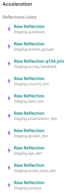
Figure 19: Reflections used by the Answer by Country execution, filtered by age, gender, and nationality

We can see that they are the first raw reflections we made in the Staging layer, not the one we have just created on top of the join.

Let’s check the query that was created to be executed on Dremio:

select `ANSWER_LABEL`,
    `ISO_CODE`,
    count(`SURVEY_ID`) as `C1`
from 
(
    select `SURVEY_ID`,
        `SURVEY_FEEDBACK_ID`,
        `ANSWER_GROUP_ID`,
        `QUESTION_ID`,
	...
        `URBANIZATION_DIM.LABEL`
    from `Processing`.`all_join`
    where ((`NATIONALITY_DIM.LABEL` = 'Austria' and `GENDER_DIM.LABEL` = 'Man') and 
`QUESTION_ID` = '1010982817') and `AGE_DIM.LABEL` = '15-24'
) as `ITBL`
group by `ANSWER_LABEL`,
    `ISO_CODE`
OFFSET 0 ROWS FETCH FIRST 1000001 ROWS ONLY

The reflection did not cover the query because we created it without using the newer filters as dimensions. One way we can solve this (although it would impact performance) is by adding all the filters to the reflection, so we end up with a reflection with the following fields:

• Dimensions
  • Survey_id
  • Question_id
  • Answer_label
  • ISO_code
  • AGE_DIM.LABEL
  • GENDER_DIM.LABEL
  • NATIONALITY_DIM.LABEL
  • QUESTION_LABEL
• Measure
  • Survey_id (count)

As we mentioned at the start of this blog post, this reflection is pretty big, and we must remember that its creation will take some time (around 30 minutes). But there is more: if our query matches this reflection Dremio will not be able to parallelise at its fullest due to the large amount of data in a single aggregation reflection.

Let’s test it:

Figure 20: Execution details for the Answer by Country chart using a single aggregation reflection with all the filters added as dimensions

Now we should check that the only reflection used was the one that we had just created:

Figure 21: Figure 21: Reflections used by the Answer by Country job after the creation of an aggregate reflection with all the possible filters

We get better performance using the general purpose raw reflections (8 seconds) than with a single huge aggregation reflection with all the filters added as dimensions (23 seconds).

This is because there are more reflections used in the job with the general purpose reflection and it is easier to parallelise the workload. Additionally, using the aggregation reflection with high-cardinality fields as dimensions (or lots of dimensions) worsens performance.

So, we can work with an aggregation reflection for the dashboards when we are not using the optional filters. However, when we want to work with lots of filters, we must avoid a single giant aggregation reflection.

As for joining the data, we have seen how a BI tool creates queries: the tasks sent to Dremio are simpler when a single table is used compared to the tasks created when letting the BI tool handle the joins by itself. Moreover, using a view to join all the table consists only of creating a virtual table of that join – the original data is left untouched and is not duplicated, but we can still work with the resulting table.

For more information about best practices for creating aggregation reflections, you can check this official Dremio blog post.

Conclusion

With this use case we have explored how to reduce costs whilst also exploiting our stored data, just by using the appropriate tools. When dealing with large datasets we cannot rely exclusively on a single BI tool and its extracts to work with our data, because sooner or later we’ll reach the limit of scalability.
 
We have also seen how we can use Dremio to query directly from data lakes, with scalability and excellent performance. More specifically, we demonstrated the proper use of reflections and concluded that we must avoid aggregation reflections with numerous dimensions. And best of all, since we are using Dremio, we can replicate the same architecture on any cloud with any BI tool!
 
We are experts at managing data and building suitable architectures no matter the field. If you have any further questions about Dremio or any doubts about building the perfect architecture to cover your data needs, do not hesitate to contact us and we’ll be happy to help!