27 Oct 2021 Real-Time Streaming Analytics with Cloudera Data Flow and SQL Stream Builder

Real-time data processing is a critical aspect for most of today’s enterprises and organisations; data analytics teams are more and more often required to digest massive volumes of high-velocity data streams coming from multiple sources and unlock their value in real time in order to accelerate time-to-insight.

Whether it is about monitoring the status of some high-end machinery, the fluctuations in the stock market, or the amount of incoming connections to the organisations’ servers,  data pipelines should be built so that critical information is immediately detected, without the delay implied by classic ETL and batch jobs.

While both IT and Business agree on the need to equip their organisation (or their customer’s) with the latest state-of-the-art solutions, leveraging the latest and greatest available technologies, the burden of the implementation, the technical challenges and the possible scarcity of required skills always falls on IT. The general consensus, in fact, is that real-time streaming is expensive and hard to implement, and requires special resources and skills.

Luckily, this has changed drastically over the last few years: new technologies are being developed and released to make such solutions more affordable and easier to implement, turning actual real-time streaming analytics into a much more realistic target to pursue within your organisation.

One of the field leaders is, of course, Cloudera. Cloudera Data Flow (CDF) is the suite of services within the Cloudera Data Platform umbrella that unlocks the streaming capabilities that you need, both on-premise or in the cloud. Specifically, the combination of Kafka, NiFi (aka Cloudera Flow Management) and the recently released SQL Stream Builder (running on Flink, available with the Cloudera Stream Analytics package) allow data analytics teams to easily build robust real-time streaming pipelines, merely by using drag and drop interfaces and – wait for it – SQL queries!

Combining the information flowing from multiple Kafka clusters with master data stored in Hive, Impala, Kudu or even other external sources has never been easier, and anybody can do it, provided they know how to write SQL queries, without needing to specialise in any other technology, programming language or paradigm.

In this article, we will introduce CDF and its different modules, and dive deep into the SQL Stream Builder service, describing how it works, and why it would be a great addition to your tech stack. We will see how easy it is to use SQL Stream Builder to query a Kafka topic, join it with static tables from our data lake, apply time-based logics and aggregations in our queries, and write the results back to our CDP cluster or to a new Kafka topic in a matter of clicks! We will also see how easy it is to create Materialized Views, allowing other enterprise applications to access data in real time with the use of REST APIs. All of this from a simple web interface, with Single Sign On, in a secure, Kerberized environment!

CDF Overview

So, what exactly is CDF? To quote the definition from the Cloudera website, CDF is “a scalable, real-time streaming analytics platform”.​

Essentially, it is a collection of services to be installed beside your existing CDP cluster, or even independently, in order to create, monitor and manage streaming and real-time applications to ingest, move, modify, enrich or even consume your data.​

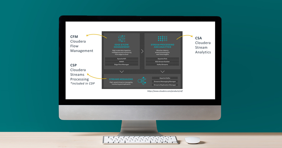
It is made up of 3 families of components, each covering a specific need.​ In the picture below, straight from the CDF website, we can see what these families are called, what services they include, and how they relate to the actual license packages that you need to acquire in order to run them.​

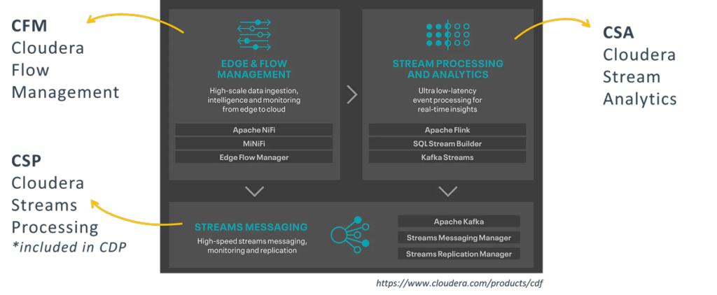
Figure 1: CDF components, as illustrated at https://www.cloudera.com/products/cdf

The first is Cloudera Flow Management, or CFM.​ CFM is used to “deliver real-time streaming data with no-code ingestion and management”.​

Practically, this translates to Apache NiFi – CFM is essentially NiFi, upgraded, packaged and integrated into the Cloudera stack, alongside other additional components which are tailored to work on edge nodes such as machines and sensors. It also includes a light version of NiFi called MiNiFi, and a monitoring application called Edge Flow Manager.​

The second package is called Cloudera Streams Messaging, initially branded as Cloudera Streams Processing (or CSP). The official definition says that it allows you to “buffer and scale massive volumes of data ingests to serve the real-time data needs of other enterprise and cloud applications”.​

In other words, it is basically Kafka, alongside two very useful new services for the management of the Kafka cluster:​

• Streams Messaging Manager, or SMM, which is a very nice UI to monitor and manage the Kafka cluster and its topics.
• Streams Replication Manager, or SRM, used to replicate topics across different clusters.​

Note that this component is actually included in the standard Cloudera Runtime for CDP Private Cloud: while it was initially branded as a separate module only, you are actually able to use it with your CDP license, without having to purchase an additional CDF license and install a new parcel.​

Finally, the last package – the one which we will focus on in the coming sections – is Cloudera Stream Analytics, or CSA.​ It is used to “empower real-time insights to improve detection and response to critical events that deliver valuable business outcomes”.​

Translated into practical terms, CSA is essentially Flink + SQL Stream Builder (SSB), and is Cloudera’s proposed solution for real-time analytics. As we said, in this article we will focus especially on SSB and test most of its capabilities.​

CSA and SQL Stream Builder

Before we describe SQL Stream Builder in detail, let’s look at why we should use CSA. As we said, Cloudera Stream Analytics is intended to “empower real-time insights”, and it includes Flink.

So, to start with, CSA offers all the Flink advantages, namely: event-driven applications, streaming analytics and continuous data pipelines,​ with high throughput and low latency,​ with the ability to write these results back to external databases and sinks.​

We can write applications to ingest real-time event streams and continuously produce and update results as events are consumed, materialising these results to files and databases on the fly; we can write pipelines that transform and enrich data while it is being moved from one system to another; and we can even connect reports and dashboards to consume all of this information with no additional delay due to batch loading or nightly ETL jobs.​

On top of this, CSA also includes SSB, which allows us to do all of this, and even more, without having to worry about how to develop a Flink application in the first place!​

The main functionality of SSB is to allow continuous SQL on unbounded data streams. Essentially, it is a SQL interface to Flink that allows us to run queries against streams, but also to join them with batch data from other sources, like Hive, Impala, Kudu or other JDBC connections (!!!).

SSB continuously processes the results of these queries to sinks of different types: for example, you can read from a Kafka topic, join the flow with lookup tables in Kudu, store the query results in Hive or redirect them to another Kafka topic, and so on.​ Of course, you can then connect to these targets with other applications to perform further analysis or visualisations of your data.​ With the Materialized View functionality, you can even create endpoints to easily consume this data from any application with a simple API call.

From a technical standpoint, SSB runs on Flink (when the queries are fired, they trigger stateful Flink jobs) and it is made up of 3 main components: the Streaming SQL Console, the SQL Stream Engine, and the Materialized View Engine.​

Hands-on Examples

Cluster Overview

Now, let’s get our hands dirty and play with CDF and SSB!

First of all, let’s take a look at what the Cloudera Manager portal looks like after installing the main CDF services:

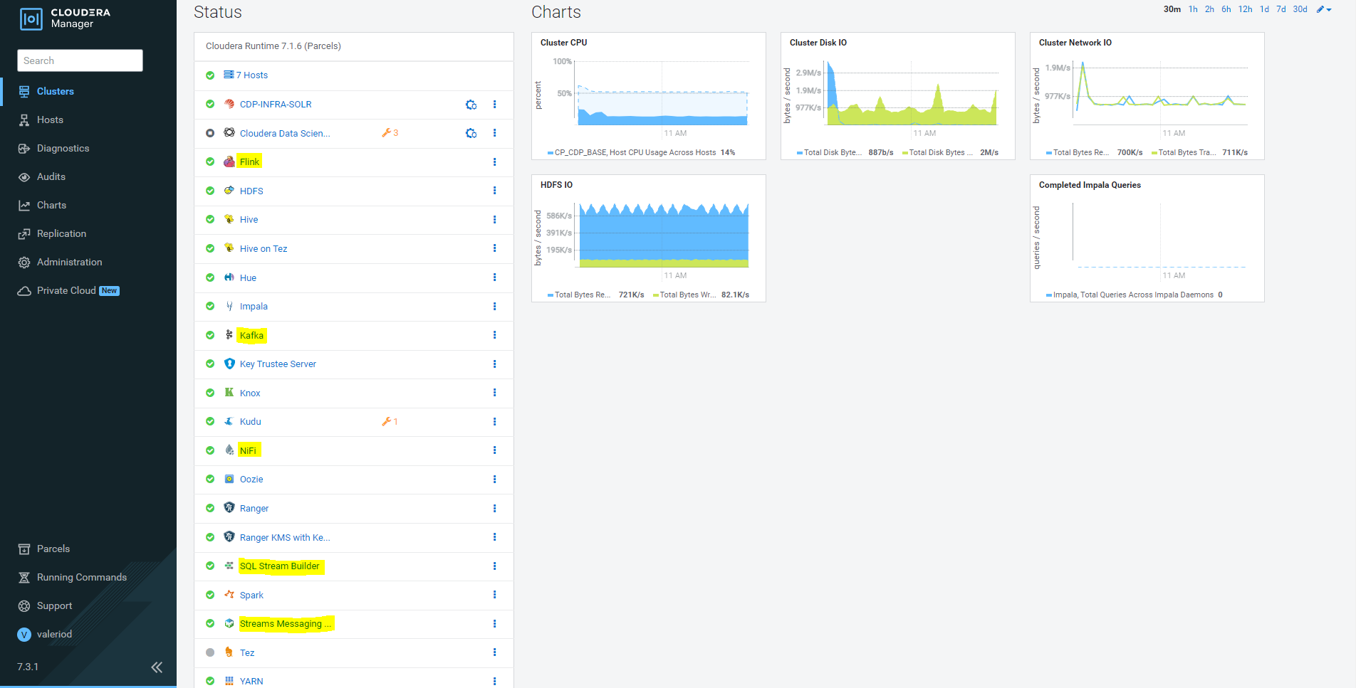
Figure 2: Cloudera Manager portal with highlighted CDF services

Note that we are using the same Cloudera Manager instance for both the CDP and the CDF services. This, however, does not have to be the case: you can, in fact, have CDF in a separate cluster if required, as long as all necessary dependencies (for example, Zookeeper) are taken care of; the actual architecture will depend on the specific use cases and requirements.

SQL Stream Builder

When we navigate to the SSB service, the Streaming SQL Console is our landing page. We can immediately see the SQL pane where we will write our queries. At the top, we can see the name of the Flink job (randomly assigned), the Sink selector, and an Advanced Settings toggle. At the bottom, we have the Logs and the Results panes (in the latter, we will see the sampled results of all of our queries, no matter the Sink we selected).

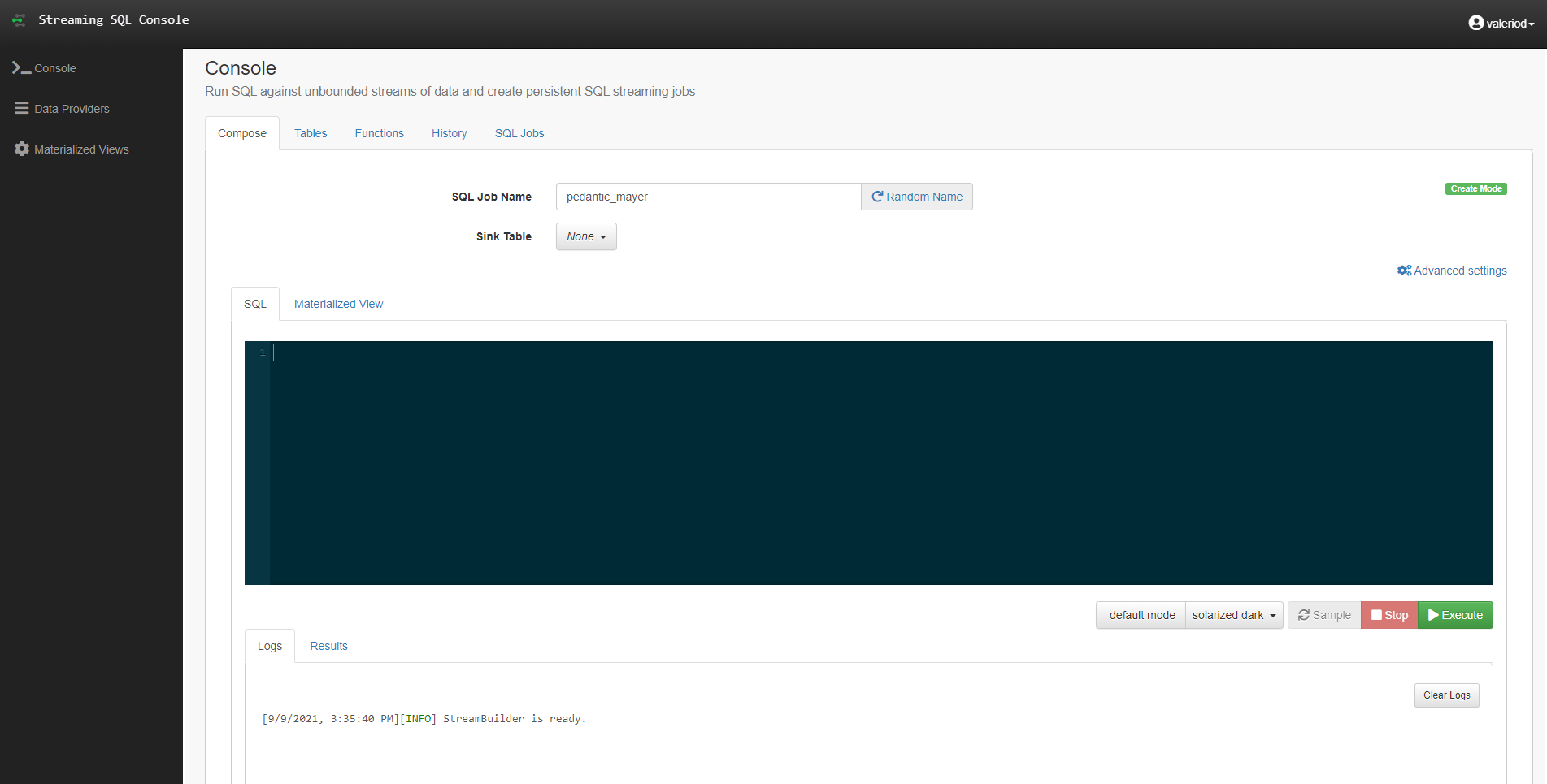
Figure 3: The Streaming SQL Console in SQL Stream Builder

On the left, we can see a navigation pane for all the main components of the tool;  we can see the Data Providers section, where we can have a look at the current Data Providers that we set up for our cluster: Kafka and Hive (automatically enabled by Cloudera Manager when installing SSB) and Kudu, which we added manually in a very straightforward process. Bear in mind that you can add more Kafka and Hive providers if necessary, and it is also possible to add Schema Registry and Custom providers, if required.

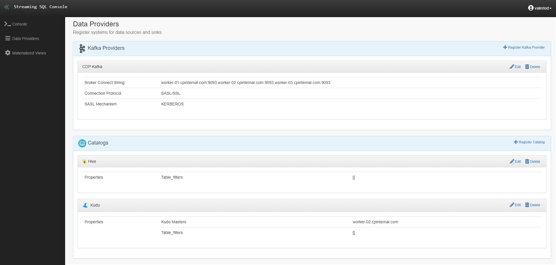
Figure 4: The Data Providers section

Back to the Console section, we move to the Tables tab, where we can see the list of available tables, depending on the Providers we configured. The first thing we notice is that we have different table types:

• Hive catalog: tables coming from the Hive Data Provider, automatically detected and not editable.
• Kudu catalog: tables coming from the Kudu Data Provider, automatically detected and not editable.
• Kafka: tables representing the SQL interface to Kafka topics, to be created manually and editable.
• Datagen/Faker: dummy data generators, specific to Flink DDL.

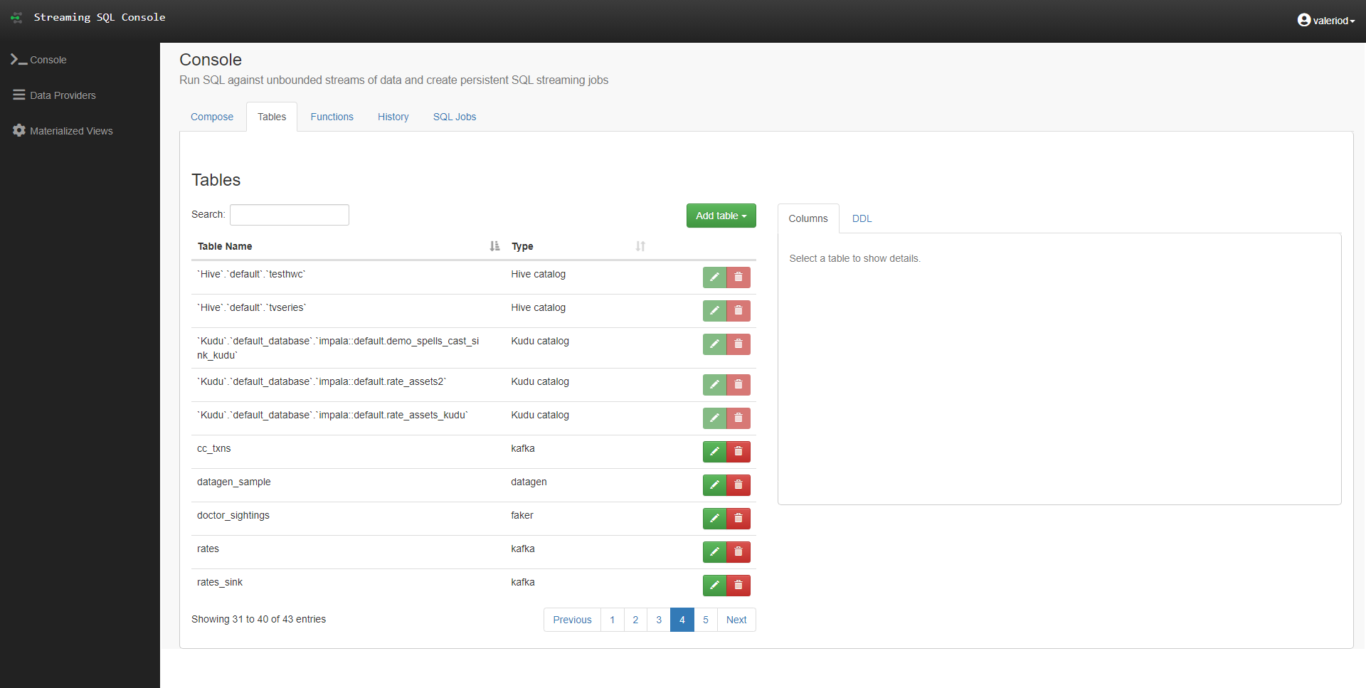
Figure 5: The Table tab in the Streaming SQL Console

The other tabs – Functions, History and SQL Jobs – respectively allow us to define and manage UDFs, check out the history of all executed queries, and manage the SQL jobs that are currently running.

Example 1: Querying a Kafka Topic

In this first example, we are going to try to query a Kafka topic as if it was a normal table. To do so, we set up a Kafka table called rates, on top of a Kafka topic with the same name. We can see the wizard that allows us to do so in the picture below. Note how you also have a Kafka cluster, a data format, and a schema, which in our case we were able to detect automatically with the Detect Schema button, since our topic is already populated with data.

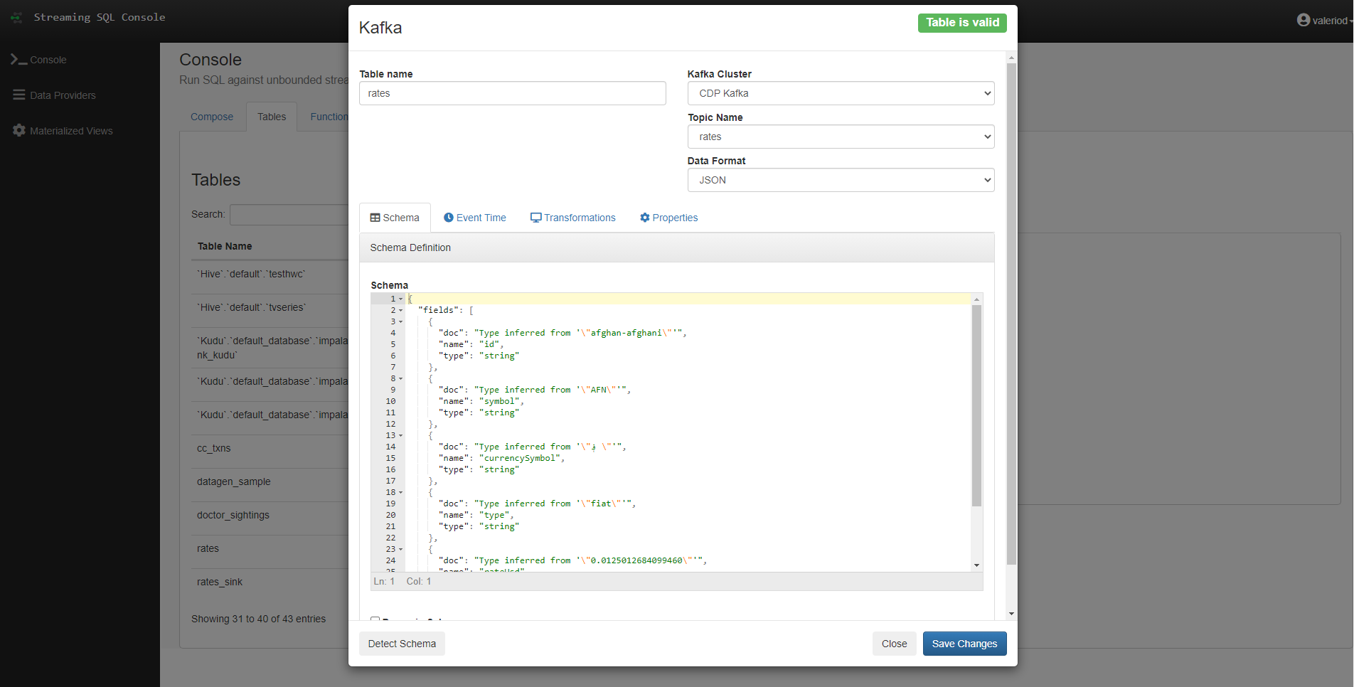
Figure 6: Wizard for the creation of a Kafka table

The topic is currently being filled by a small NiFi pipeline that continuously pulls data from a public API providing the live rates in USD of many currencies, including cryptos. Using Streams Messaging Manager (the new UI to monitor and manage the Kafka cluster) we can easily take a look at the content of the topic:

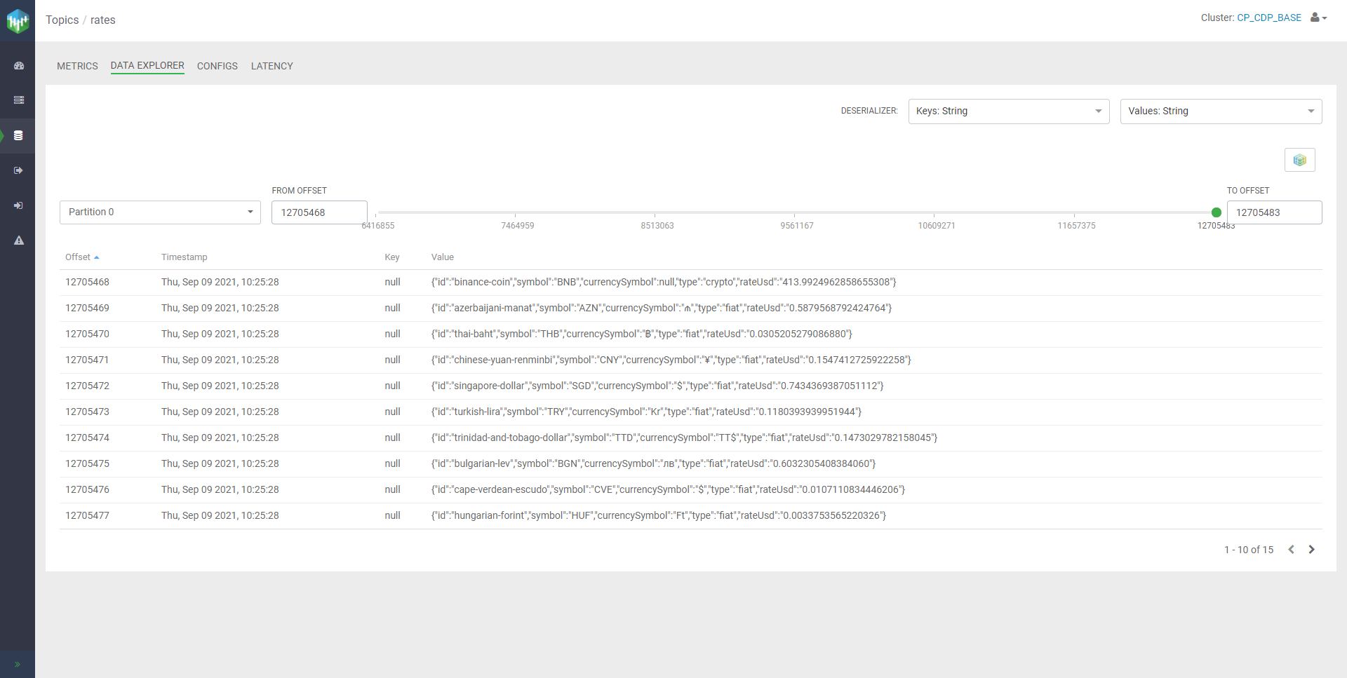
Figure 7: View of the Data Explorer in SMM, with a sample of messages in the ‘rates’ topic

As we can see, all messages are in JSON format, with a schema that matches the one automatically detected by SSB.

Going back to the Compose tab, we now run our first query:

select * from rates 

As you can see, it is just a simple SQL query, selecting from rates as if it was a normal structured table. Since Sink is set to none, the result is simply displayed in the Results pane, and is continuously updated as more data flows into the topic.

Figure 8: Sampled results of the query on the ‘rates’ topic

Of course, we could also edit the query, just as we would do for any other SQL statement. For example, we could decide to select just a few of the original columns, apply a where condition, and so on.

If we look at the Logs tab, we can see how we effectively started a Flink job; this job is also visible in the Flink dashboard, to be monitored and managed just like any other Flink job. Furthermore, as we have already mentioned, all the SSB jobs can also be managed from the SQL Jobs tab in the SQL Console, alongside the History tab where we can see information about past executions.

Example 2: Joining Kafka with Kudu

We have seen above how to query unbounded data ingested in Kafka, a very cool feature of SSB. However, what is actually even cooler about this new tool is that it allows you to mix and match unbounded and bounded sources seamlessly.

In this new example, we join the live currency rates with some currency master data that we have in a pre-populated Kudu table.

select
	r.id,
	a.`symbol`,
    	a.`rank`,
	a.name,
	r.currencySymbol,
	r.type,
	r.rateUsd,
    	r.eventTimestamp,
	a.explorer
from ( select
      id,
      symbol,
      currencySymbol,
      type,
      CAST(rateUsd as DOUBLE) as rateUsd,
      CAST(eventTimestamp as TIMESTAMP) as eventTimestamp
      from rates
  ) r join `Kudu`.`default_database`.`impala::default.rate_assets_kudu` a
on r.id = a.id
where a.`rank` <=5

As you can see, this is nothing but SQL, yet we are joining a streaming source with a batch table! And we did not have to write a single line of code or worry about deploying any application!

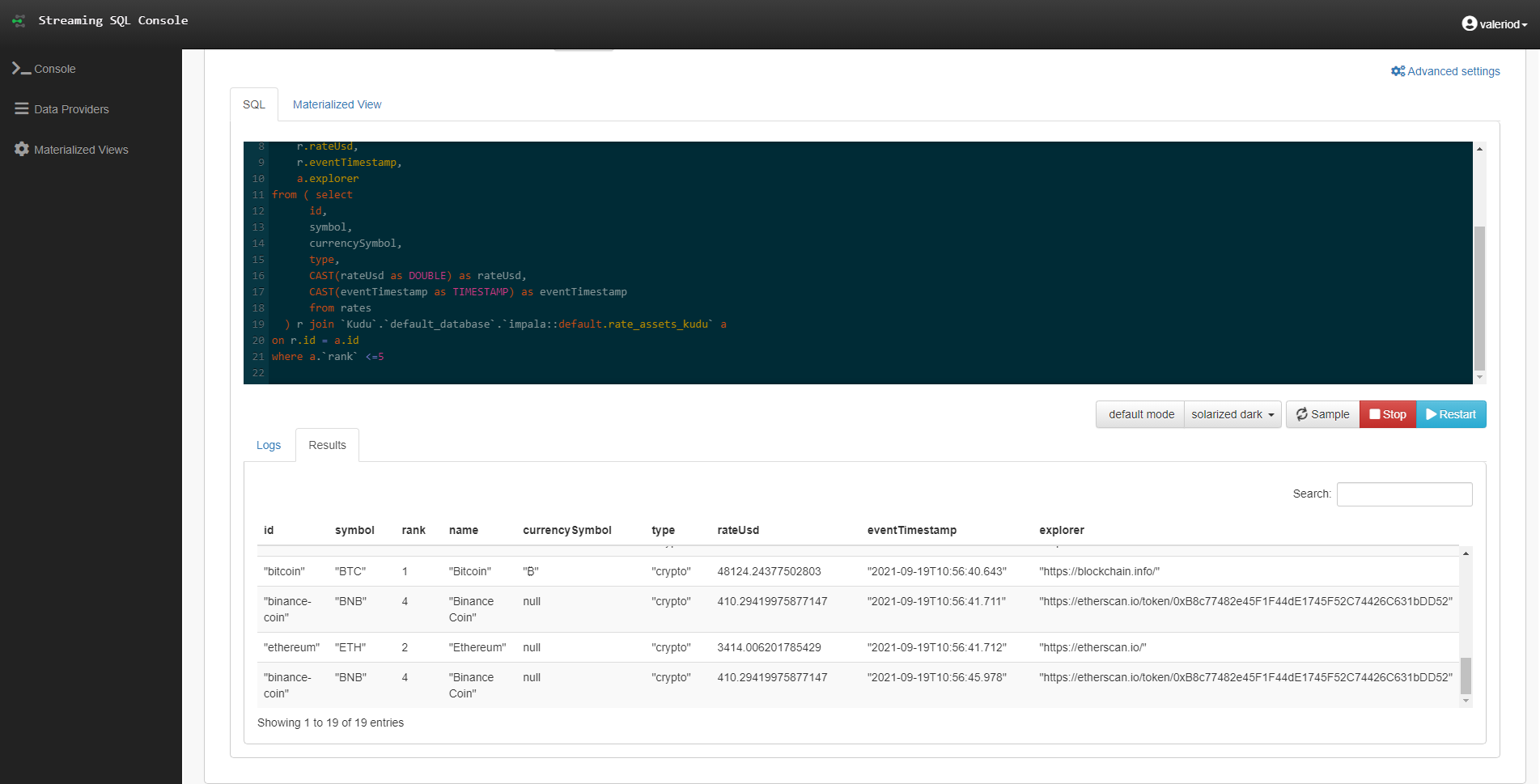
Figure 9: Joining a Kafta topic with a Kudu table

Example 3: Storing Results to Hive

So far, we have only been displaying the results of our queries on the screen. However, you may wonder – can I store this somewhere? Luckily, the answer is yes: this is possible thanks to the Sink. In fact, we can select any of the tables defined in our Tables tab as Sink, provided (of course) that their schema matches the output of our query.

In this example, we run a query that is very similar to the previous one, but with 3 main differences:

• The Sink is a previously created Parquet table.
• the lookup data is in Hive and not in Kudu.
• there is a “FOR SYSTEM_TIME AS OF PROCTIME()” clause in the Join statement.

select
	r.id,
	a.`symbol`,
    	a.`rank`,
	a.name,
	r.currencySymbol,
	r.type,
	r.rateUsd,
    	r.eventTimestamp,
	a.explorer
from ( select
      id,
      symbol,
      currencySymbol,
      type,
      CAST(rateUsd as DOUBLE) as rateUsd,
      CAST(eventTimestamp as TIMESTAMP) as eventTimestamp
      from rates
  ) r join `Hive`.`default`.`rate_assets_hive_txt` FOR SYSTEM_TIME AS OF PROCTIME() AS a
on r.id = a.id
where a.`rank` <=5;

While the change from Kudu to Hive is only to showcase another possible combination that SSB allows, the real difference in this case is in that extra clause in the join: that little piece of query is needed in order to allow Flink to effectively commit all the little partitions that it will create in the Hive table location. Without this, it would just keep adding data to a single partition without ever finalizing, and our Sink table would always be empty when queried.

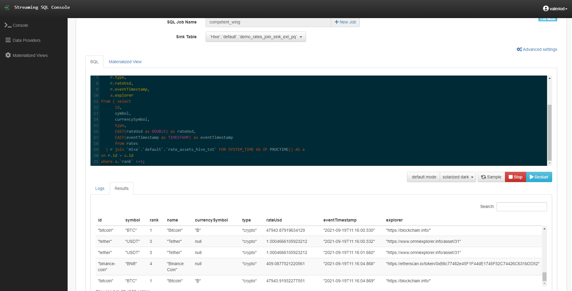
Figure 10: Using a Parquet table as Sink for a real-time join query

If we query the Sink table while the job is running, we can see that it is actually being populated in real time by the output of our query:

Figure 11: Sample of the Parquet table being populated in real time

Example 4: Applying a Window function

In the previous examples, we have run pure SQL queries, with the exception of the clause required to properly store the results back in HDFS. However, as mentioned, we can also use Flink-specific functions to perform certain time-based logics.

In this example, we use the WINDOW function, which allows us to group records and calculate aggregated metrics for a specific interval of time:

select
	id,
	symbol,
	currencySymbol,
	type,
	CAST(rateUsd as DOUBLE) as rateUsd,
	MIN(CAST(rateUsd as DOUBLE)) OVER last_interval AS min_rateUsd,
	MAX(CAST(rateUsd as DOUBLE)) OVER last_interval AS max_rateUsd,
	CAST(eventTimestamp as TIMESTAMP) as eventTimestamp
FROM rates where id = 'dogecoin'
WINDOW last_interval AS (
  PARTITION BY id
  ORDER BY eventTimestamp
  RANGE BETWEEN INTERVAL '1' MINUTE PRECEDING AND CURRENT ROW 
)

The above query will look very familiar to those of you who know how windowing functions work in SQL. We are partitioning the real-time rates by the currency ID, ordering by the record timestamp, and specifying an interval of 1 minute: essentially, for every currency, we are selecting the records that arrived in the previous minute and we are calculating the maximum and minimum rate in this interval. To help us understand the output, we also filter by one specific currency, in order to be able to see its evolution and notice how the aggregated measures change in time.

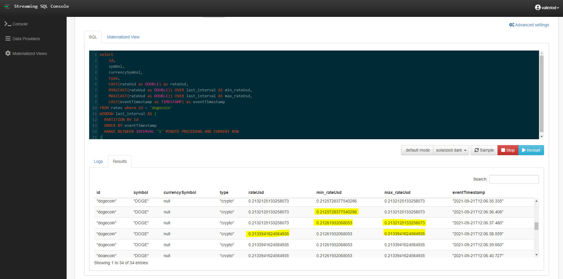
Figure 12: Results of a query using the Window function

Note how both the minimum and maximum rate changed in a couple of seconds, according to the dogecoin rates received in the previous minute.

Example 5: Redirecting Results to a Kafka Topic

Not only we can store the results of our query in a table, but we can also redirect them to a new Kafka topic. We will now try to do so, using the same query as in the previous example.

First of all, we need to create a topic. In Streams Messaging Manager this is a very easy task: in the Topics section, we click on “Add New” and select the details for our topic. Note that in order for the Flink job to be able to effectively write the results there, we need to select the delete clean-up policy. We call the topic rates_window_sink.

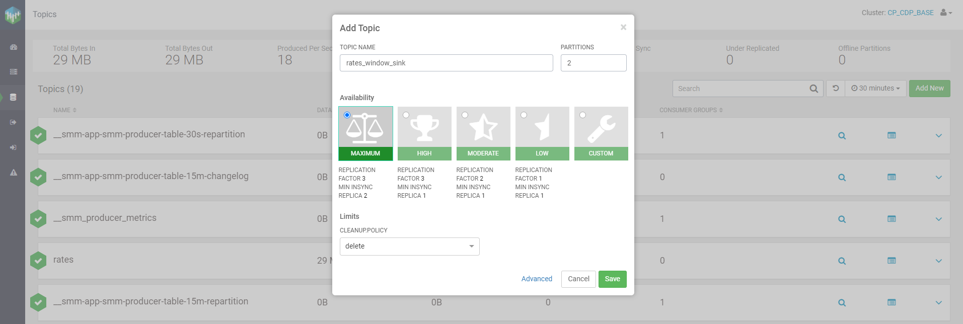
Figure 13: Creating a new topic in SMM

Now that we have our topic, we need to create a Kafka table on top of it in SSB. Back to the Streaming SQL Console, we go to the Tables tab, and we add a new Kafka table. We assign a name, select the Kafka Cluster, select the topic we just created, our preferred format, and then we click on the Dynamic Schema checkbox. This will allow us to store messages with any schema in this table, without worrying about their consistency. However, notice how once we have done so, SSB tells us that this table can be only used as a Sink!

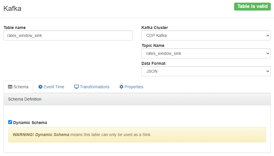
Figure 14: Creating a Kafka table for a Sink with Dynamic Schema

Once our table has been created, we run the previous Window query again, this time selecting our new Sink. Once the job has started, we go back to SMM to monitor our new topic, and we can see how data is effectively flowing in in real time as it is processed by the SSB query.

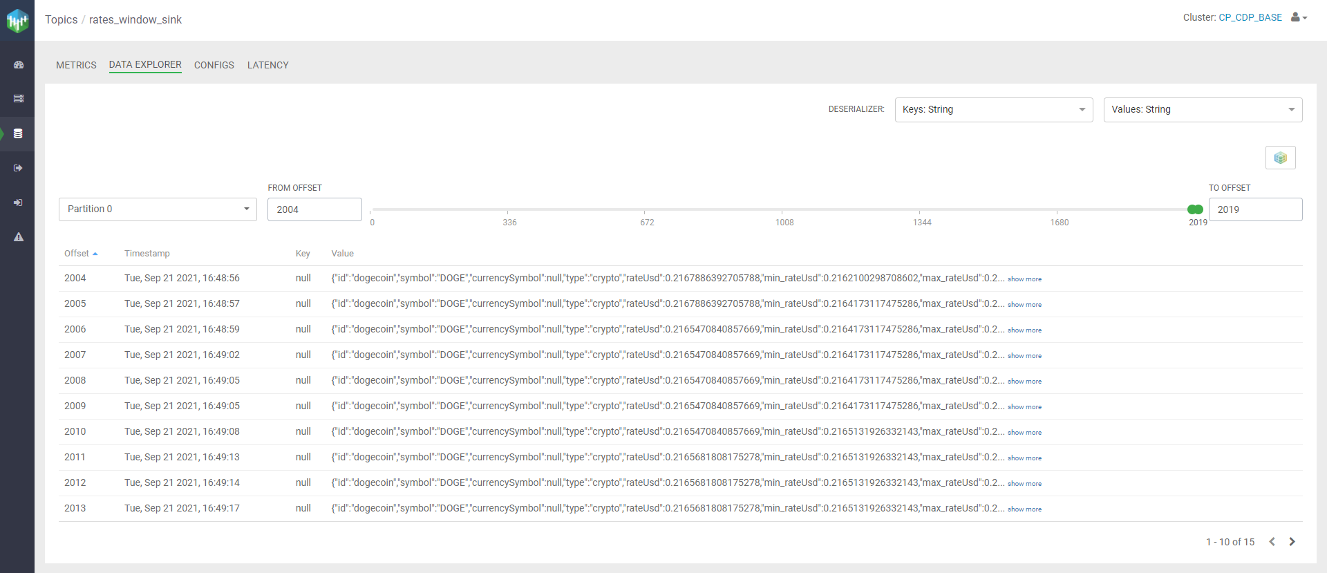
Figure 15: View of the Kafka Sink in SMM

Example 6: Materialized View

Finally, in this last example, we will demonstrate the Materialized View functionality. Materialized Views can be thought of as snapshots of the query result that always contain the latest version of the data, represented by key. Their content is updated as the query runs, and is exposed through a REST endpoint that is associated to a key and can be called by any other application. For this example, we used the following query:

SELECT
	wizard,
	spell,
	CAST(COUNT(*) as INT) AS times_cast
FROM spells_cast
WHERE spell IN ('Expecto Patronum')
GROUP BY
	TUMBLE(PROCTIME(), INTERVAL '10' SECOND),
	wizard,
	spell

This query pulls data from a faker table, which is a type of connector available in Flink that allows us to create dummy data following certain rules. In our case, each row of the dummy dataset indicates a spell cast by a wizard . In our query, which uses another Flink function called TUMBLE, we want to count the number of times that a specific spell has been cast in the last 10 seconds by every wizard.

To create a materialized view for this query, we move to the pane of the Console tab, we select wizard as Primary Key, and we create a new API Key (if we did not have one already). As you can see below, there are more settings available. When we have finished, we click on “Apply Configurations”:

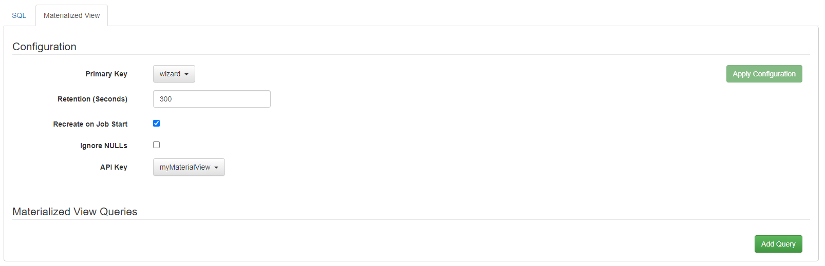
Figure 16: Creating a Materialized View

At this point, the “Add Query” button is enabled. This allows us to define API endpoints over the SQL query that we defined. Potentially, we can define multiple endpoints over the same result. We create one query by selecting all fields, and we click on “Save Changes”:

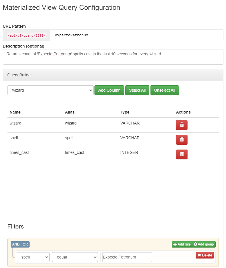
Figure 17: Creating an endpoint for a Materialized View

For every query we create, we get a URL endpoint. We can copy it and paste it in our browser to test our materialized view. If the job is running, we will obtain a JSON with the content of our view, as defined in our endpoint.

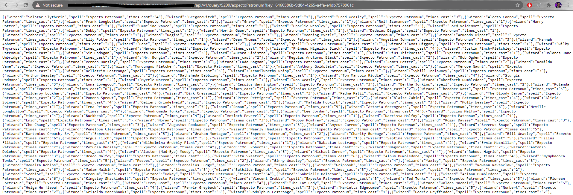
Figure 18: Result of our Materialized View endpoint

We are now free to take this endpoint and use it in any other application to access the results of our query in real time!

Conclusion

In this article, we have demonstrated how easy it is to build end-to-end stream applications, processing, storing and exposing real-time data without having to code, manage and maintain complex applications. All it took was a bit of SQL knowledge and the very user-friendly UIs of SQL Stream Builder.

We have also seen how useful some of the new CDF services are, particularly Streams Messaging Manager, a powerful solution to “cure the Kafka blindness”, allowing users to manage and monitor their Kafka cluster without having to struggle with Kerberos tickets and configuration files in an OS console.

In general, CDF has become a really comprehensive platform for all streaming needs. At ClearPeaks, we can proudly call ourselves CDF and CDP experts, so please contact us with any questions you might have or if you are interested in these or other Cloudera products. We will be more than happy to help you and guide you along your journey through real-time analytics, big data and advanced analytics!

If you want to see a practical demo of the examples above, head to our YouTube channel and watch a replay of our recent CoolTalks session on this topic. And do consider subscribing to our newsletter so that you don’t miss exciting updates!