
16 Jul 2020 Running TeraSort on Hortonworks and Isilon OneFS
We recently came across an interesting situation with one of our customers and we think it will be of interest for other Big Data engineers and administrators who need to work on a similar deployment – we are talking about a Hortonworks Data Platform (HDP) 3.1 platform in which the storage layer is managed by Dell EMC Isilon OneFS and not by regular HDFS. If you do not know what Isilon OneFS is and how it relates with Hadoop, please read the Annex at the bottom of this blog article. From now on, we assume you are familiar with Isilon OneFS as storage layer for Hadoop.
After completing the HDP+Isilon platform installation and configuration for our customer, we wanted to benchmark it, and one of the many tests we ran was the TeraSort suite.
The TeraSort suite is arguably the most popular and widely used Hadoop benchmark – note it is only meant to benchmark the core of Hadoop (MapReduce, YARN and HDFS). Hence it is irrelevant if your workload involves other services like Spark, HBase, Kafka, etc. The TeraSort suite consists of three map/reduce applications:
- TeraGen is a map-only program that generates random unsorted data and stores it in HDFS. Each generated record has 100 bytes and consists of a randomly generated key and an arbitrary value. When running the application, you can control the number of records that will be generated and the number of HDFS files in which they will be stored. TeraGen is mostly a HDFS write performance test.
- TeraSort is a map/reduce program that reads the unsorted data generated by TeraGen and sorts it. Both input (unsorted) and output (sorted) data are stored in HDFS. TeraSort also makes extensive use of intermediate data stored in the local disks. Therefore, TeraSort will test HDFS read/write, local disks read/write, inbound and outbound networks, CPU and memory.
- TeraValidate is a map/reduce program that reads the output from TeraSort and validates it is sorted. TeraValidate is mostly a HDFS read performance.
Note that the TeraSort suite is available in the source code of Hadoop – you can find it in hadoop-mapreduce-examples.jar. Much has been written about the TeraSort suite: on Cloudera Community you can find a few articles by Sunile Manjee in which he runs the suite in Bigstep and AWS EMR, and he goes into details of the parameters used in those runs in this other blog article. Michael G. Noll also offers in his web page an interesting blog entry about TeraSort and also other Hadoop benchmarks (TestDFSIO, NNBench and MRBench). Finally, also check out the blog article by Claudio Fahey, especially relevant since it also discusses running the TeraSort suite on Isilon (though the article is dated from 2015 and back then EMC had not been acquired by Dell).
The goal of our TeraSort benchmark exercise was to check the overall platform performance, so we wanted to maximize resource utilization during the execution of the various programs. We ran the suite with different dataset sizes (10GB, 100GB, 1TB, 10TB) and we also ran with different numbers of users (1, 5, 10); in the process we found some interesting issues that we want to share. For the sake of brevity, we will only discuss 2 benchmark scenarios: (a) 1 user – 1TB; (b) 10 users – 1TB each.
TeraGen
The very first step is to run TeraGen to generate the unsorted data. As mentioned above, TeraGen is a map-only program, meaning that it only runs mappers, not reducers. To run TeraGen in single-user scenario and for a size of 1 TB we first tried:
time hadoop jar /usr/hdp/3.1.0.0-78/hadoop-mapreduce/hadoop-mapreduce-examples.jar teragen -Dio.file.buffer.size=131072 -Dmapreduce.map.java.opts=-Xmx1536m -Dmapreduce.map.memory.mb=2048 -Dmapreduce.task.io.sort.mb=256 -Dyarn.app.mapreduce.am.resource.mb=1024 -Dmapred.map.tasks=330 10000000000 /user/oscar/terasort-input-1000000000000 > /home/oscar/teragen100000000000.log 2>&1
We followed the recommendations from Claudio Fahey’s article and set the mapper memory to 2GB; we also used the settings he recommended. The only thing we changed was the block size, which in our case was 128MB and could not be changed (due to Isilon); we also specified a different number of mappers. We used 330 mappers (each using 2GB) in order to ensure most of our cluster resources were used (at that point the YARN capacity we could use was 6 nodes x 128GB). The number of mappers also determines the number of output files, since each mapper will write exactly one file on HDFS. For optimal performance, choose a number of mappers (in combination with the memory allocated per mapper) that is close to the total capacity of YARN. The parameter that controls the size is set to 10000000000 (10 zeros) and this indicates the number of 100-byte records that will be generated. Therefore, the size of the generated dataset will indeed be 1 TB (“12 zeros” bytes). Note we ran the command with “time” to measure the exact execution time and we also redirected both standard output and error to a log file for a thorough analysis later.
We ran a single 1TB TeraGen in 197 seconds using 100% of the memory of the cluster for most of the time (we checked the YARN Resource Manager UI and monitored the resources used during the execution). The aggregated resource utilization was 91079556 MB of RAM and 22069 vCores (x seconds) so on average we used 450 GB of RAM and 112 vCores. So, our first TeraGen result was already quite decent!
Afterwards, we also ran 10 TeraGen in parallel with 10 different users. We used a number of mappers that was smaller in every run (33) so that we could guarantee the overall YARN capacity was not over-requested. Of course, we could also leave each parallel TeraGen with 330 mappers and YARN would handle over-allocation using pre-emption but this would blur our performance observation (pre-emption is what happens when a user is running a job and another user starts a new job, and YARN queue policy enforces that the first user must free resources so that the second user can use them – that causes some jobs in the first user to be killed by YARN and restarted transparently by the user).
Our TeraGen runs, both single-user and multi-user, did not produce many surprises in the various tests we did, and all outcomes were as expected. So, let’s move on to TeraSort, the most interesting part.
TeraSort
After running TeraGen with single and multiple users we wanted to run TeraSort for the generated datasets.
Single TeraSort
In our single-user scenario we first tried to run the following command, also based on Claudio Fahey’s recommendations:
time hadoop jar /usr/hdp/3.1.0.0-78/hadoop-mapreduce/hadoop-mapreduce-examples.jar terasort -Dio.file.buffer.size=131072 -Dmapreduce.map.java.opts=-Xmx1536m -Dmapreduce.map.memory.mb=2048 -Dmapreduce.map.output.compress=true -Dmapreduce.map.output.compress.codec=org.apache.hadoop.io.compress.Lz4Codec -Dmapreduce.reduce.java.opts=-Xmx1536m -Dmapreduce.reduce.memory.mb=2048 -Dmapreduce.task.io.sort.factor=100 -Dmapreduce.task.io.sort.mb=768 -Dyarn.app.mapreduce.am.resource.mb=1024 -Dmapreduce.job.reduces=165 -Dmapreduce.terasort.output.replication=1 /user/oscar/terasort-input-1000000000000 /user/oscar/terasort-output-1000000000000-test > /home/oscar/terasort100000000000-test.log 2>&1
So, we specified 2GB for both mappers and reducers, indicated that the map outputs (intermediate data) will be stored with Lz4 compression, and fine-tuned the sorting parameters. We specified just 165 reducers in our first attempt so as to be conservative. Note that you cannot manually specify the number of mappers – this is automatically determined by dividing the total size of the input files by the split size which by default is the HDFS block size, so in our case it was around 8000 mappers (1TB / 128MB). The two final parameters specify the input and output HDFS folders respectively. As we did with TeraGen, we used “time” to measure execution time and we redirected all logging to a file for posterior analysis.
With the above parameters the TeraGen took over 2 hours to complete. This is longer than what we would consider acceptable, even considering the conservative parameters we set (namely the number of reducers). It took some time to work out what was happening.
Before we dive into the solution, let’s look at a simplification of what the TeraSort job did on the various hardware components of the HDP+Isilon platform – this will help to understand the bottleneck we found. First, the Map phase started – each mapper read a block from Isilon (via network) and wrote an intermediate file on the local disk of an HDP node. Then, when about the 70% of the mappers were done, the Reduce phase started. The Reduce phase has three subphases: Shuffle, Sort and Reduce. First, the Shuffle sub-phase read data from local disks and shuffled it to other local disks using the network. Second, the Sort sub-phase also read from and wrote to local disks. Finally, the Reduce sub-phase read mostly from local disks and wrote the output to Isilon.
When monitoring the job, we realized that during the Map phase, even though in principle there were almost 8000 mappers that should run, we could only see around 7% of the cluster was being used (only around 10 YARN containers) while during the Reduce phase we could see much higher utilization (around 70% of the cluster was used). The Map phase was taking forever to complete, but once it completed, the Reduce phase was fast. So, there was something odd happening during the Map phase.
We checked the logs and there were indeed almost 8000 mappers being requested and they eventually ran, but there were never more than 10 of them running at the same time. In principle, YARN should use all the available resources in the cluster – no one else was using it. Why was YARN not giving more resources to the Map phase of our TeraSort?
We found that the problem was that the mappers were too fast: each mapper was completing its work within a few seconds (less than 10 ). Actually, it was taking the same time for YARN to launch 10 new mappers as the previous 10 mappers to complete their work, so effectively there were never more than 10 mappers running. Still, there were almost 8000 mappers, and if only 10 were running in parallel and each was taking 10 seconds, well, there you have our 2 hours.
Once we had identified this issue, we had to think out how to fix it. After some deliberations, we finally realized the best approach was to have less mappers and give each one more work to do. But how? Remember that the number of mappers is determined by the total size of the dataset divided by the split size which is set by default to the block size. So, let’s just use a higher block size! However, in our case changing the block size was not possible. What can we do then? Wait! Let’s change the split size! There is a parameter (mapreduce.input.fileinputformat.split.minsize) to change the split size that each mapper will use to fetch the data from HDFS (Isilon in our case), so we used that parameter to ensure a split was mapping to more than just one block. For example, the command below sets a split to be 12 times a block size – so, roughly each mapper will read 12 times more data and will be 12 times slower which should give YARN enough time to spawn all containers, and we will have 12 times less mappers (we also changed io.file.buffer.size but it is not clear that was necessary):
time hadoop jar /usr/hdp/3.1.0.0-78/hadoop-mapreduce/hadoop-mapreduce-examples.jar terasort -Dio.file.buffer.size=393216 -Dmapreduce.map.java.opts=-Xmx1536m -Dmapreduce.map.memory.mb=2048 -Dmapreduce.map.output.compress=true -Dmapreduce.map.output.compress.codec=org.apache.hadoop.io.compress.Lz4Codec -Dmapreduce.reduce.java.opts=-Xmx1536m -Dmapreduce.reduce.memory.mb=2048 -Dmapreduce.task.io.sort.factor=100 -Dmapreduce.task.io.sort.mb=768 -Dyarn.app.mapreduce.am.resource.mb=4096 -Dmapreduce.job.reduces=165 -Dmapreduce.terasort.output.replication=1 -Dmapreduce.input.fileinputformat.split.minsize=1610612736 /user/oscar/terasort-input-1000000000000 /user/oscar/terasort-output-1000000000000-test > /home/oscar/terasort100000000000-test.log 2>&1
With this change, TeraSort went from over 2 hours to less than 20 minutes (1035 seconds) and the YARN UI was showing utilization of more than 70% most of the time. Actually, the aggregated resource utilization was 401500198 MBxSecond and 97609 vCoresxSecond so on average we used 380 GB of RAM and 95 vCores.
Multiple TeraSort
Once we managed to get one TeraSort to go as fast as we wanted, we decided to test 10 TeraSorts in parallel, each executed by a different user (if you are wondering how we did this, we used the command-line screen quite extensively).
We restricted the number of reducers (from 165 to 16) per job and went ahead with the execution. The number of mappers was still automatically decided (though we could control it with the split size) so we had to accept there would be some YARN pre-emption here and there.
We ran the test and observed multiple errors in the logs. To our surprise, we found that the local disks, which were used to handle intermediate data, were not capable of managing the workload and were timing out few tasks. Some mappers and reducers were being killed because local disks were too slow to complete their IO operations. This was not happening in a single TeraSort. When we had one single TeraSort, all the jobs running on the cluster were mostly stressing the same hardware components at the same time. First, during the Map Phase all the YARN containers were running mappers that read Isilon and wrote to local disks, then, during Shuffle and Sort, most containers were first reading from and then writing to local disks and finally, during Reduce, most containers were reading from local disks and writing to Isilon. However, when we had multiple TeraSort jobs running in parallel, the jobs were in different phases, which caused the local disks to bottleneck since they were too slow to handle all the requested IO operations of different natures.
Since in the customer’s platform the HDFS is managed by Isilon, the HDP nodes were configured with only 2 SATA devices (in RAID-1) for the intermediate data storage. We found out that for workloads that are heavy in the use of intermediate data (such as multiple TeraSorts in parallel) this setting is not ideal, and we should consider increasing the number of local disks. Of course, in practice we do not expect to be running 10 1TB TeraSorts in parallel any time soon, since the cluster will be used for workloads that will leverage the memory (Spark) more, so for now we do not expect we will hit this bottleneck soon. But if our customer experiences this gain, they will know what to do.
TeraValidate
After running TeraSort we ran TeraValidate to validate all data was properly sorted. In general, if TeraSort finished properly there is not much to de here, and TeraValidate will basically only assess the read performance from HDFS, Isilon in our case.
So, again following the recommendations of Claudio Fahey, we ran TeraValidate with:
time hadoop jar /usr/hdp/3.1.0.0-78/hadoop-mapreduce/hadoop-mapreduce-examples.jar teravalidate -Dio.file.buffer.size=131072 -Dmapreduce.map.java.opts=-Xmx1536m -Dmapreduce.map.memory.mb=2048 -Dmapreduce.reduce.java.opts=-Xmx1536m -Dmapreduce.reduce.memory.mb=2048 -Dmapreduce.task.io.sort.mb=256 -Dyarn.app.mapreduce.am.resource.mb=1024 -Dmapred.reduce.tasks=1 /user/oscar/terasort-output-1000000000000 /user/oscar/teravalidate-output-100000000000 > /home/oscar/teravalidate100000000000.log 2>&1
We specified 2GB for mappers and reducers and set the rest of parameters like in Claudio’s blog. As usual, we just added the “time” and log redirection. Note TeraValidate will use as many mappers as TeraSort had reducers, so in our case it was 165. The TeraValidate for a single user completed in 339 seconds and used on average 70% of the cluster.
Like in TeraGen, the execution of TeraValidate did not produce any surprises in the single and multi-user scenario, and all results were as expected.
Conclusions
In this blog article we described two issues we faced while running TeraSort for single and multiple users, benchmarking scenarios on an HDP platform in which the storage layer is managed by Isilon OneFS instead of regular HDFS. The bottom line: use higher block sizes or split sizes if your TeraSort mappers are too fast; and properly size your intermediate data stores (local disks) for your expected workloads even if using decouple storage with Isilon OneFS.
We have been helping our customers with troubleshooting, fine-tuning and optimizations of their Big Data platforms and workloads for quite some time now, so if you need our help in these regards, do not hesitate and contact us.
Annex
Our customer’s platform is made up of HDP 3.1 and Dell EMC Isilon OneFs. Most of the services that are shipped in HDP are installed and configured: YARN, MapReduce, Hive, Tez, Pig, Spark, HBase, Phoenix, Druid, Storm, Oozie, Zeppelin, Kafka and Sqoop; security is provided by Kerberos (identity management by Active Directory), Ranger, Knox and Atlas; and, as usual, Ambari and Zookeeper keep the zoo in order. Figure 1 depicts the services available in HDP 3.1 and indicates which ones have been installed and enabled for our customer.
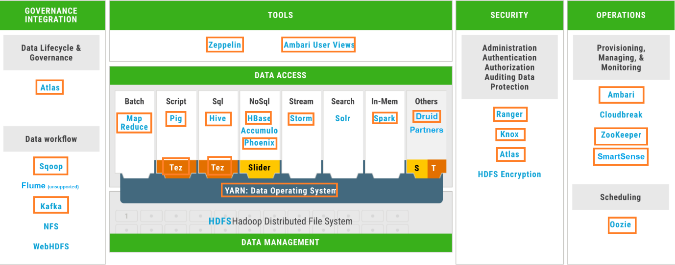
Figure 1: HDP 3.1 distribution. Orange-boxed services are the ones installed and enabled for our customer
As you may have noticed, we have not mentioned HDFS; this is because, as commented, in this deployment the storage layer is managed by Dell EMC Isilon OneFS, not the regular HDFS. So, in this architecture storage and compute are decoupled, i.e. the resources used for storage and for compute are in different machines, pretty much like we have in modern Big Data Cloud architectures. Check some of our previous blogs for examples of these modern Big Data Cloud architectures: in this blog you can see the Azure Data Lake Storage in action in conjunction with Azure Databricks (and also compared with other engines available in Azure), while in this other blog you can see AWS S3 in conjunction with AWS Glue. Both examples in Azure and AWS have decoupling of storage and compute – the most obvious benefit of such decoupling is that you can scale each part independently. When storage and compute are coupled, often the case in on-prem deployments, you usually need to scale both storage and compute at the same time, even if you really only need to increase one of the two, basically because the hardware is the same – though in some cases you can add more disks to a node if you have physical drive slots available or more RAM if you have physical memory slots available; adding more cores to a physical (i.e. not virtual) server is not something easily done.
We believe decoupling storage and compute which is the norm in Cloud will also become the norm in on-prem Big Data deployments. You can find a proof of the last statement in the inner details of Cloudera Data Platform (CDP) which we dissected in a previous blog article as well as in our talk in the Big Things Conference in November 2019. CDP is the new product from Cloudera after the merger with Hortonworks, and not only does it combine the former Cloudera Distribution of Hadoop (CDH) with HDP, but it also improves the resulting product. One of the novelties of CDP is that it incorporates by design the separation of compute and storage in both Cloud and on-prem deployments. On Cloud (CDP Public Cloud) storage is provided by a logical layer within CDP called Data Lake which relies on Azure Data Lake Storage or AWS S3. In on-prem (CDP Data Center) we have, at the very least, the separation at logical level – a base cluster has HDFS and auxiliary services and one can create Data Hub clusters for compute (how the logical level maps to physical is of course something we can control).
Just in case you are a bit lost with what the decoupling of storage and compute actually means in an on-prem deployment, please have a look at Figure 2 and Figure 3.
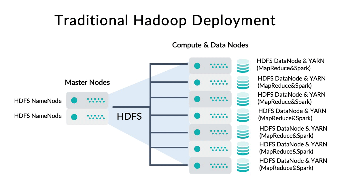
Figure 2: Traditional Hadoop deployment (coupled storage and compute).
In traditional Hadoop clusters, as depicted in Figure 2, we have a master node (or more than one if we want High Availability) in which we run the HDFS master process (HDFS NameNode), and then we have a few worker nodes in which we have the actual data as well as the HDFS worker processes that will handle it (HDFS DataNode). The same worker nodes are used for compute purposes and in them we also install the services in charge of data processing (YARN, MapReduce, Spark, etc.). This configuration offers the benefit of “Data Locality”, meaning that when whatever engine (MapReduce or Spark) needs to process the data, YARN (the resource negotiator) can try to ensure that data is processed by cores and memory of the same node in which the data is stored (otherwise data will need to be sent to another node via the local network).
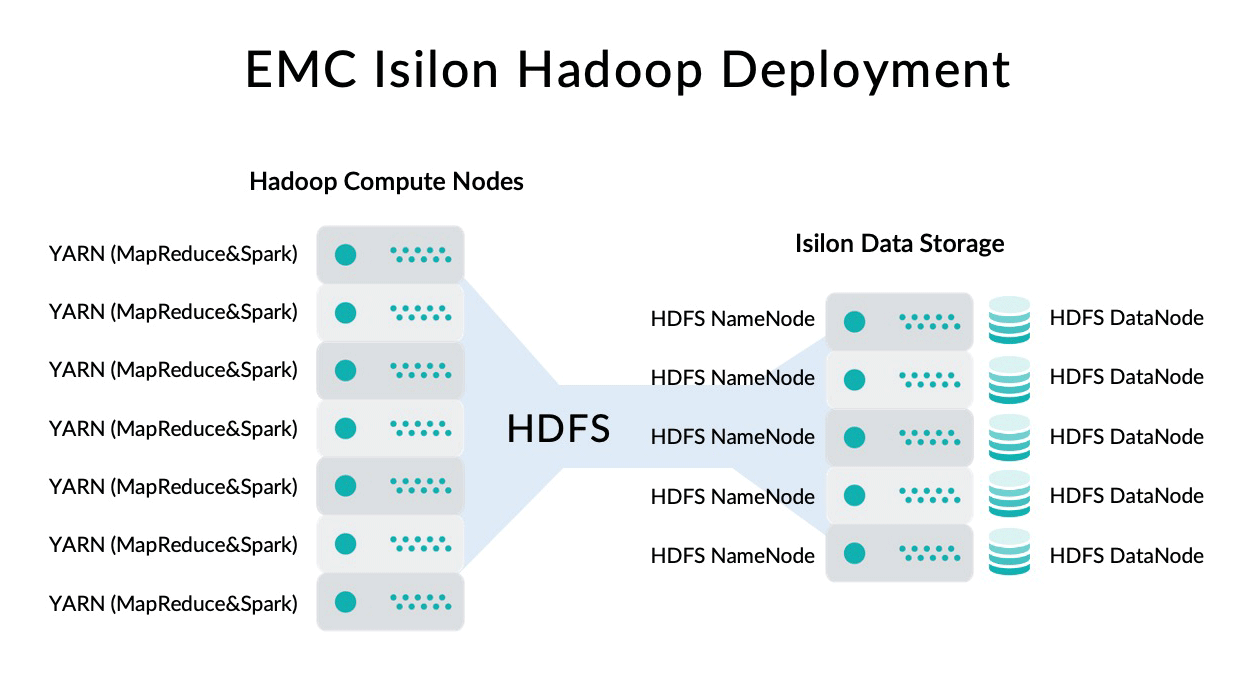
Figure 3: EMC Isilon Hadoop Deployment (decouple storage and compute).
As depicted in Figure 3, Dell EMC Isilon OneFS provides a scale-out network-attached storage (NAS) platform which is independent from the Hadoop cluster and could therefore scale independently. Isilon OneFS provides access to its data using a HDFS protocol. Isilon OneFS itself is also a cluster of nodes and all nodes provide NameNode and DataNode HDFS functionality so it is highly available; so data remains in Isilon nodes and the Hadoop cluster provides the computing power to process it. The downside, of course, is that network usage will be much more intense than in the traditional Hadoop deployments (Figure 2) since Data Locality is just not possible here, and all data needs to travel from Isilon to Hadoop nodes when it needs to be used. However, if the network deployment is properly scaled and the throughput is high enough this drawback is compensated for (note this is the daily bread and butter of Cloud architectures and they are, after all, very successful).
In either case, be it traditional or with Isilon, the end user just sees an HDFS that they can use, without even needing to know if it is a local HDFS or an Isilon. We could say that the HDP+Isilon architecture of our customer is ahead of its time since it already incorporates decoupling of storage and compute which is the trend that modern Big Data architectures are following – storage and compute decoupling is already the norm in Cloud and, as we said earlier, the latest developments in Cloudera seem to indicate that it will also become the norm on-prem.