09 Dec 2020 Data Masking and Row Level Security on CDP with Ranger

In a recent blog we explained how to spin up a CDP cluster in Azure and how to deploy a Data Engineering Data Hub on top of it.

This time, we are going to use the Data Hub and explore one of the most important and utilized features in every data platform implementation: authorization in Hive with Ranger.

As you may know, Ranger is a new addition to the Cloudera universe; it was first included in HDP and replaced Sentry after Hortonworks was acquired by Cloudera.

It is a very powerful and easy-to-use tool that provides authorization mechanisms on CDP: it allows the implementation of all different kind of access policies to data on CDP services, like allowing or denying access to HDFS folders, Hive tables, HBase tables, Kafka topics, etc. Furthermore, it also allows the application of fine-grained Row Level Security (RLS) and Data Masking policies.

We are often asked by our clients about RLS and Data Masking, and we will try to answer the most common questions in the following sections. Specifically, we will demonstrate the following scenarios:

• Data Masking.
• Filtering masked data.
• Joining over masked data.
• RLS over masked data.

1. Setting up Hive tables

Hive is immediately available as soon as your Data Engineering cluster is deployed; no additional configuration is required. Just click on the Hue service and you will be redirected to the Hue page, where you can start loading your data. How to load data in Hive is outside the scope of this article; for this exercise, we used the GUI to manually load two similar tables of dummy data: mock_data_1 and mock_data_2.

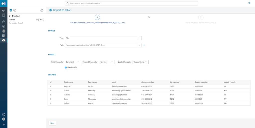
Figure 1: Manually loading data in Hive through Hue’s GUI.

Once the tables have been loaded, we can proceed to query them. Since we haven’t defined any rules yet, we will be able to select all of the columns without any restrictions.

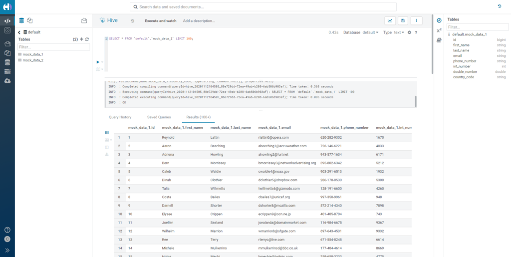
Figure 2: How our mock data looks without any policies.

2. Applying Data Masking rules

Now that our Hive tables are ready, let’s move to Ranger and define some rules.

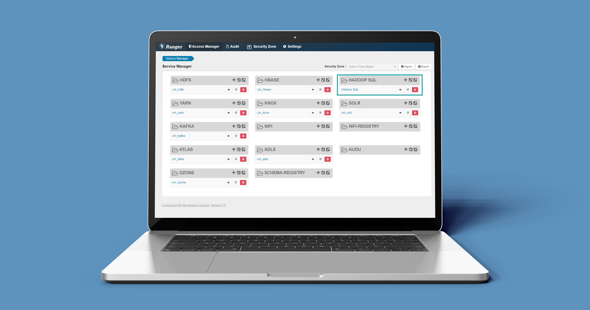
The Ranger landing page presents different sections, one for every service for which rules can be defined. In our case, we want to go to the Hadoop SQL service.

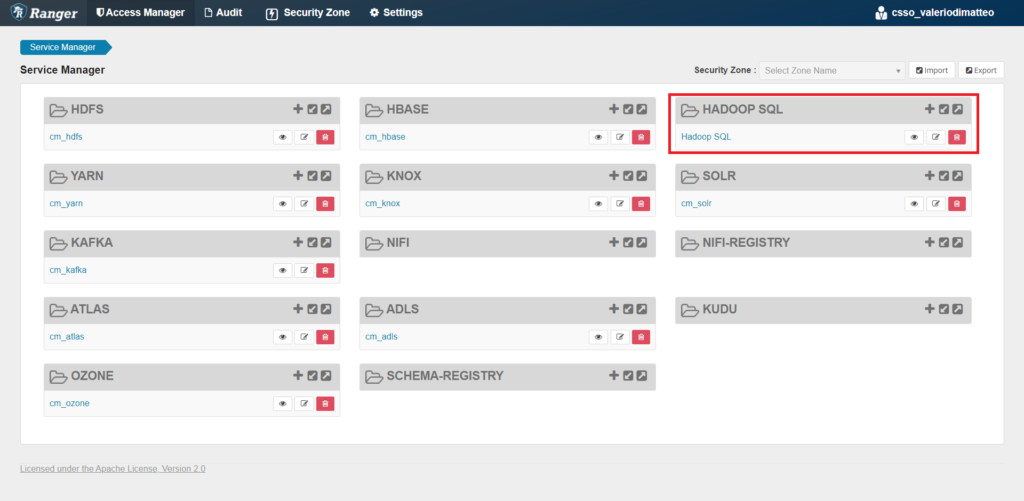
Figure 3: Ranger’s landing page and the Hadoop SQL section.

First of all, you can see we have different sections depending on the type of policy we want to apply: Access, Masking, Row Level Filter. We are going to start with some Masking rules – let’s go there and click on Add New Policy.

When we create a new policy, we have to define a series of parameters:

• Policy Type:
• Policy Name: a name to recognize our policy. If we plan to create a lot of them, it’s a good idea to come up with a name pattern.
• Policy Label: a label to apply to our policy. If we create a lot of policies, this is useful when searching for policies that conceptually belong to the same group (like ‘region’ or ‘department’).
• Hive database: the database that contains our data. You can select one or all (*).
• Hive table: the table that contains our data. You can select one or all (*).
• Hive column: the column that we want to mask. You can only select one.

Below, you can select which users the new rule will be applied to: you can select Roles, Groups and specific users; you can then select the type of access we are referring to. As we are applying a masking rule, we can only choose SELECT. Finally, select the type of masking rule; there are many options, and below we can see the complete list, as taken from the CDPdocumentation here.

• Redact – mask all alphabetic characters with “x” and all numeric characters with “n”.
• Partial mask: show last 4 – show only the last four characters.
• Partial mask: show first 4 – show only the first four characters.
• Hash – replace all characters with a hash of entire cell value.
• Nullify – replace all characters with a NULL value.
• Unmasked (retain original value) – no masking is applied.
• Date: show only year – show only the year portion of a date string and default the month and day to 01/01.
• Custom – specify a custom masked value or expression. Custom masking can use any valid Hive UDF (which returns the same data type as the data type in the column being masked).

3. Masking single columns

3.1. Strings

In our first example, we apply the Redact option over the email column of the table mock_data_1.

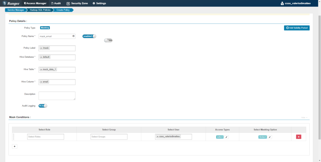
Figure 4: Creation of a Data Masking policy for column email.

We save the rule, then go back to Hue and query the table again. What we see is quite different from before: the email column has been redacted, so we are not able to determine the real value anymore. This is only valid for my user, because this is the only user we selected when creating the rule. If any other user comes in and queries this table, they will see the original values of the email column (provided, of course, they have access).

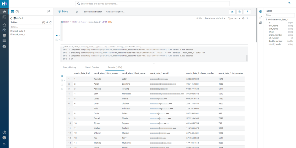
Figure 5: Querying a redacted string column.

Now let’s try another type of masking: let’s change the type to Hash. Again, we query the same data, but the result is different: instead of seeing the original email values, we see a list of long hashed strings. There is a big difference here: hashing is consistent and maintains the uniqueness of the data, something that redaction is generally not able to do.

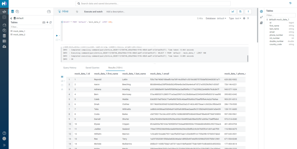
Figure 6: Querying hashed data.

3.2. Numbers

So far, we have tried different masking options on strings. Let’s see what happens if we want to apply masking rules over numerical values.

Go back to Ranger, and then add a rule to redact the column int_number. As the name suggests, this column is an integer.

Figure 7: Creation of a Data Masking policy for column int_number.

Based on the description that Cloudera provides for the Redact option, this should turn every digit into a 1. Go back to Hue and query the data again. Effectively, each value of int_number is now substituted by digits of 1.

Note: this only applies for integers. For doubles and floats, the result would be a NULL.

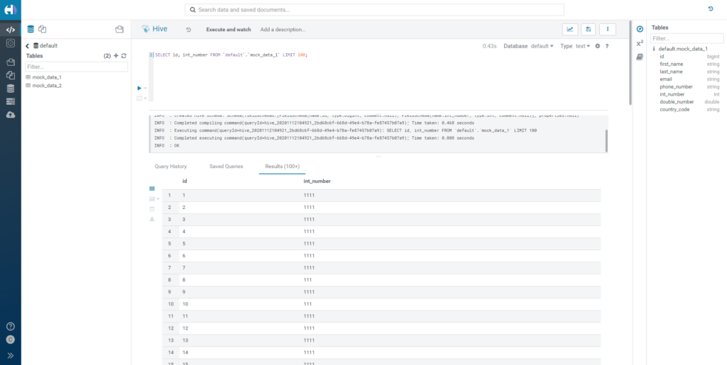
Figure 8: Querying redacted numerical data.

Now let’s now change the rule from Masking to Hash. This time, we don’t get the same result: every number has been replaced by a NULL value. This is because the hashing function returns a string, but our column type is an integer, so it’s not applicable. This is worth noting, since it is something that does not immediately come to mind and might generate unexpected results.

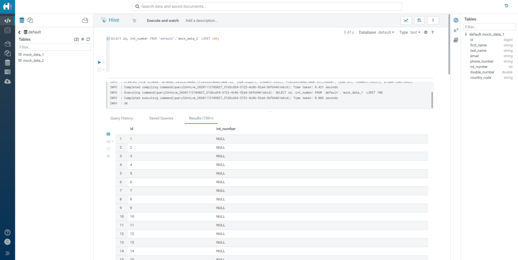
Figure 9: Outcome of hashing numerical data.

3.3. Custom

Finally, Ranger allows  you to use custom functions to mask your data. You can use any Hive function or UDF, as long as the output type is the same as the input. You can specify the formula by selecting Custom and by writing it in the textbox that appears. To refer to the column itself in the formula, you have to use {col}.

For example, we apply this rule to the column first_name:

translate(translate(initcap(reverse({col})),’o’,’0′),’e’,’E’)

The output is a reversed version of the original first_name, with a few substitutions in the characters.

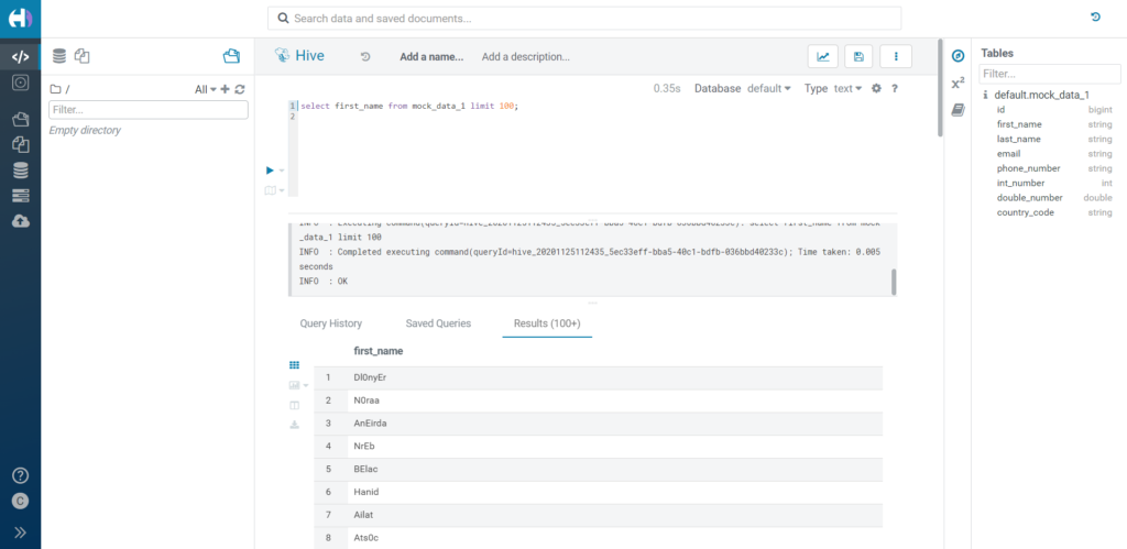
Figure 10: Applying a UDF transformation in a Custom Data Masking policy.

4. Filter with masked data

Now that we have seen a few examples of different types of masking rule, let’s look at how they behave when we filter the data.

4.1. Redact

As a first test, let’s see what happens if we filter a redacted value. We create a masking rule over the country_code column, and we try to filter it by both one original value and its redacted version.

The filter will be applied over the redacted value as if they were normal strings in this case, so we will get 0 or all rows depending on whether we use the original or the redacted version in the filter condition.

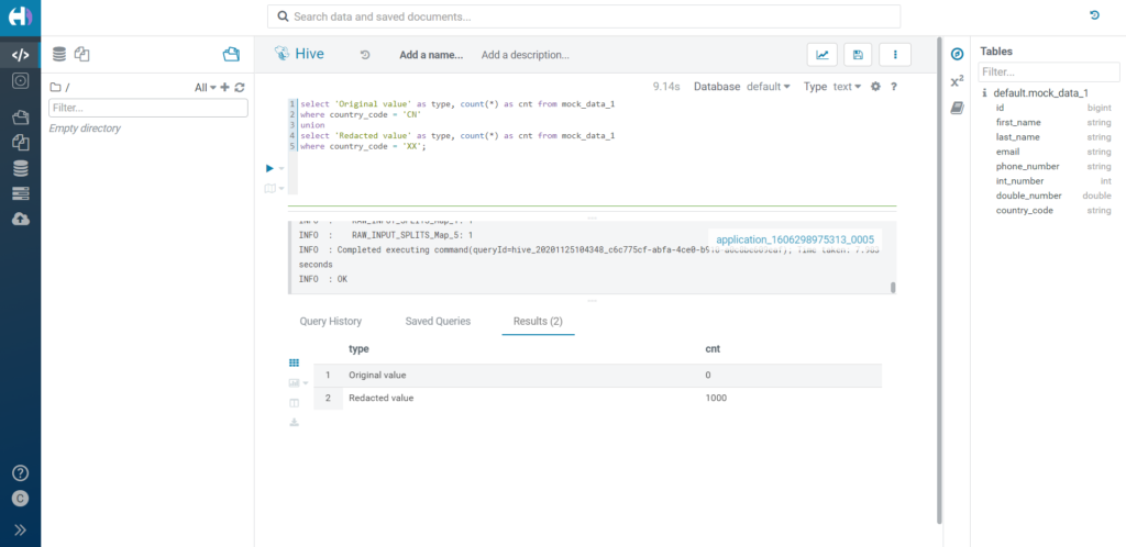
Figure 11: Filtering over redacted data.

Similarly, a redacted integer value is effectively filtered using its redacted counterpart, made of digits of 1. As for doubles and floats, we have seen how the redaction turns them into NULLs, so the filter would behave accordingly.

4.2. Hash

Let’s try to filter over a hashed value. What happens in this case is that the condition of the filter is compared to the hashed value, not the original one.

For example, if we filter by country_code = ‘CN’, we will find 0 results, while all values will be selected correctly if we actually filter by the hashed value.

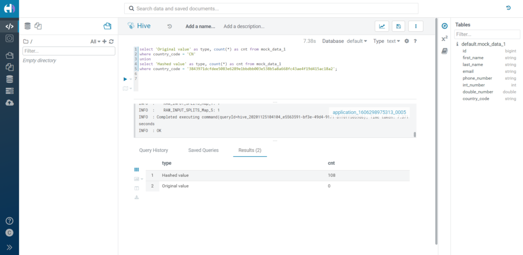
Figure 12: Filtering over hashed data.

4.3. Custom

Finally, let’s see how the filters apply to custom-masked data. We can use the same rule we applied when we demonstrated the custom masking type and try to filter for both the new and original value. As you would expect, the row is correctly picked up by the filter on the masked value.

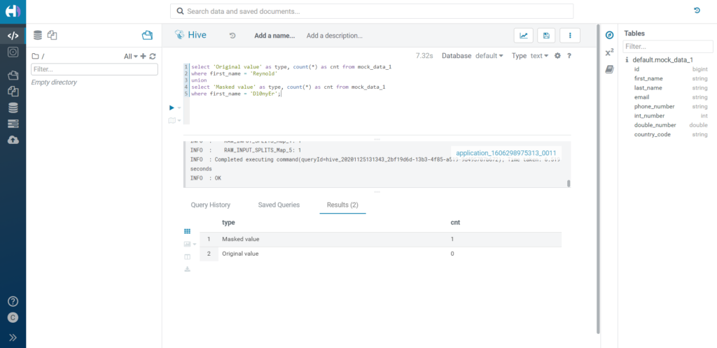
Figure 13: Filtering over custom masked data.

5. Joining over masked data

So far, we have tested some basic scenarios and evaluated the main characteristics of masking rules. Now, let’s answer one of the questions we get asked most often by our clients: can we join over masked data?

First of all, this is a question which can be answered from the technical side, but also from a business and/or Infosec perspective. Whether or not your users should be able to join over masked data depends on what levels of information you want to share. As we have said, redacting, for example, does not keep the uniqueness of the data, while hashing does and is a consistent function. This, alone or when joined with other tables, can cause some information to be inferred, when perhaps it should not be. What happens, for example, if we hash the Gender column of a table? We’ll get two different results, and immediately be able to tell whether two people are of the same gender or not; the amount of values typically used to indicate gender is also quite limited, so we could even infer the original value after few brute force attempts. With redaction, we won’t be able to do this. Hashing also allows us to group data correctly, even though we can’t see the original value of the group; furthermore, if we join this information with some external master data, we might be able to make hypotheses which we’re not supposed to (for example, guess the State of a person based on the demographic distribution of our data correlated with public data of State populations).

Potentially, however, joining over masked data offers huge benefits, since it allows for total flexibility over our data: the possibility to easily and immediately apply multiple masking rules based on user, group, role and tag; no need to store multiple copies of the data; immediate availability of masked data that does not have to pass through external masking, hashing or tokenization processes, thus greatly improving our time-to-value.

Assuming that all of this is clear to you and that your organization has thoroughly assessed the various possible scenarios before deciding on the authorization rules for every user and table, let’s start by answering the question from a purely technical angle.

5.1. Redact

Let’s begin with a basic test: joining over redacted columns. We would expect this join not to produce any meaningful result, as the purpose of the redaction is not to disclose any information.

In fact, the outcome is as expected. In our case, we redacted the column country_code in both tables, mock_data_1 and mock_data_2: the column has the same format in both tables, so it is redacted with the same value (‘XX’). The result of this join is equivalent to a Cartesian product: not very useful. Of course, if the two columns had different formats and different redacted values, the join result would be a smaller (possibly empty) set.

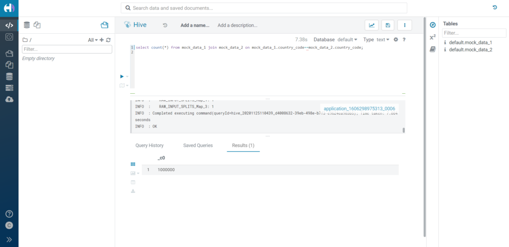
Figure 14: Joining over redacted data.

A join between redacted integers would produce a similar result. In this case, however, we might have different formats in the values (depending on the digits of the number), so the output would probably be smaller than a Cartesian product. As for doubles and floats, we have mentioned how the redaction turns them into NULLs, so the join wouldn’t make much sense.

5.2. Hash

Now let’s try to perform a join over hashed columns. Before starting, we must count the highest values of the country_code column: in both cases, China is the most common value, with 173 and 185 occurrences respectively for tables mock_data_1 and mock_data_2, so we can expect these two values to correspond to the same hashed value. In fact, this is exactly what happens when we join both tables over the hashed country_code column.

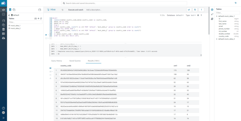
Figure 15: Joining over hashed data.

This means that joining is indeed possible with hashed data.

5.3. Custom

As a last example, we’re going to join the two tables over a custom-masked value. Again, we apply a rule on both country_code columns, but this time we make it custom and we specify the following formula:

lcase(reverse({col}))

When grouping and joining the two tables, we can see how the top row  once again shows 173 and 185 occurrences in mock_data_1 and mock_data_2 respectively. This means our data was correctly joined using the actual masked value, and still produced a meaningful result.

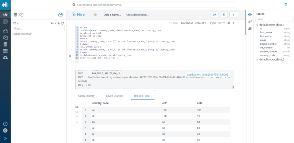
Figure 16: Joining over custom masked data.

6. RLS with masked data

So far, we have seen how all the masked values were correctly picked up by filters and join. The natural question at this point is: if we have applied a Row Level Security rule over the original value, will it be broken if we apply a masking rule? Let’s find out.

In Ranger, RLS rules are applied from the Row Level Filter tab of the Hadoop SQL policies. Their definition is very similar to the masking rule, except that:

• There is no need to define any column.
• There is no type selection, but only a textbox in which we apply the expression. (exactly as we would write it in a where clause). Remember that the expression is inclusive.

First of all, we apply a redaction rule over our country_code column. This means, as we have already observed, that all its values will be represented by the string ‘XX’.

Now we apply our first RLS under the Row Level Filter tab, so that our user can see everything but the rows related to China; we do so by specifying the following expression in the Row Level Filter box of our policy:

country_code <> ‘CN’

Now we count the rows we have access to. We know already, from our previous tests, that mock_data_1 contains a total of 173 rows with country_value equal to ‘CN’. The total number of rows in the table is 1000, so we expect to see 827 rows if our RLS rule is correctly applied despite the masking rule being enabled. In fact, this is exactly what we see.

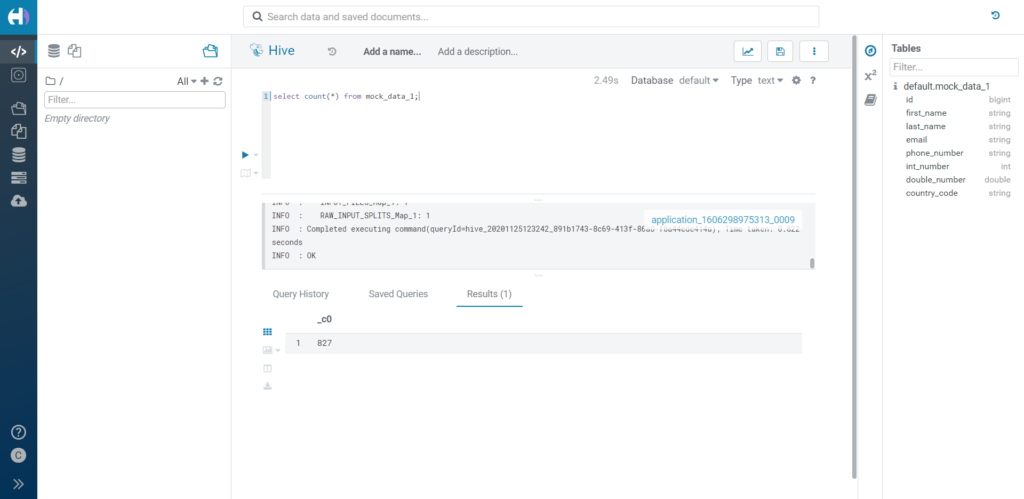
Figure 17: RLS over masked data.

The exact same outcome is obtained if the masking rule is a hash instead of a redact, or a custom rule, and so on, no matter the column type of the masked value.

Conclusion

We’ve taken a pretty deep dive into Ranger’s capabilities over Hive, and we’ve seen how to apply most of the masking rules, and how they integrate perfectly with RLS policies. This is possible because RLS is applied before the query output is generated, and masking is only applied at the end of the process. They can live together happily!

As we mentioned, bear in mind that masking is a very delicate process from the business and Infosec perspective. The benefit of Ranger is that it allows a very simple and flexible way to define rules at the lowest level of granularity, so no matter what your requirement is, you will most probably find a way to apply it through Ranger. In this sense, custom masking offers a great deal of possibilities. Furthermore, we can also apply rules based on Atlas tags, leveraging this other great feature for even more combinations (this is accessible by clicking on Access Manager in the top bar, and selecting Tag Based Policies).

Finally, it’s worth noting how all of the policies are applied under the ‘Hadoop SQL’ service, and not under ‘Hive’. This means that Impala will also follow them in exactly the same way, as well as Spark (provided you use the Hive Warehouse Connector to access the tables). And what’s more, remember that Ranger is a Data Lake service, so all the rules we define will be applied across every Data Hub or Experience that we spin up! This is the power of SDX.

Next steps

In our last article  we saw how to set up a Data Engineering cluster in CDP on Azure. Today, we’ve gone a step further, demonstrating how to apply Ranger rules over Hive tables, thus answering some of the most common questions that arise when designing a data platform in CDP.

In the next articles, we will look at other basic CDP services, to showcase their capabilities and highlight the differences with respect to the legacy versions of CDH and HDP. Stay tuned!

If you have any questions, doubts, or are simply interested in discovering more about Cloudera and CDP, do not hesitate to contact us at ClearPeaks. Our certified experts will be more than happy to help you and guide you in your journey towards the ultimate Enterprise Data Platform!