07 Jan 2021 Extreme Performance Boost for KNIME Spatial Processing

KNIME Spatial Processing nodes help in reading and writing spatial data from various formats and provide standardized transformation, filtering, and visualization features. In this article, we discuss the use of KNIME’s spatial processing nodes in an example use case of tagging a taxi location (by using its latitude and longitude) to a particular geo fence area. We will also take you through the approach of how we have utilized several KNIME features along with Python integrations to deliver an enormous performance boost.

1. First Approach: Using KNIME standard Spatial Processing nodes

*KNIME Spatial Processing nodes can be installed from the following update site: http://update.knime.com/community-contributions/4.2

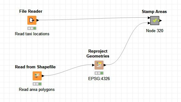
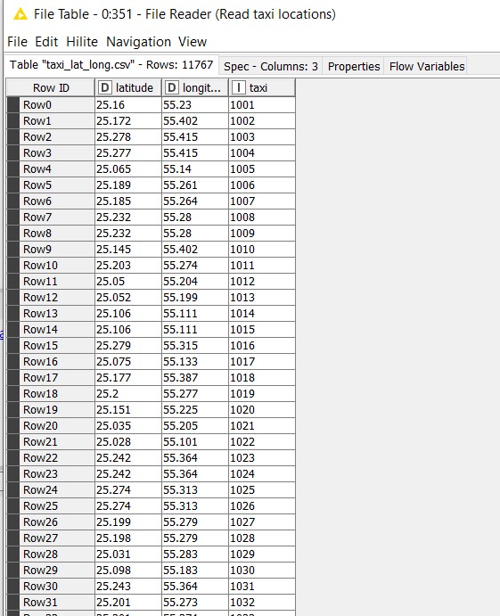
In this example, we take a sample dataset having taxi locations (taxi code with latitude and longitude information, ‘taxi_lat_long.csv ‘). Based on the latitude and longitude values, we aim to identify the geo fence area each taxi is currently located in.

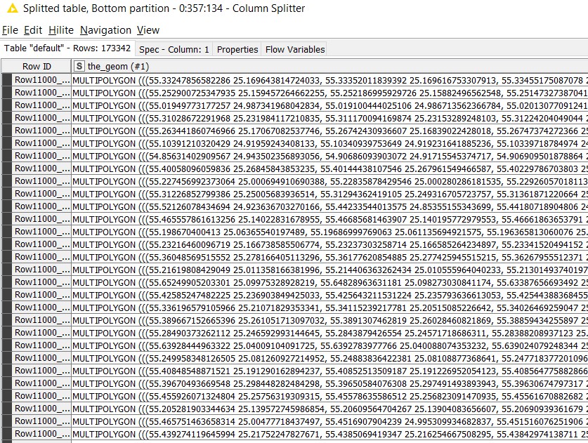
The ‘Read from Shapefile’ KNIME extension reads spatial features (geometries) from a shapefile. It accepts any geometry type: points, lines, polygons, multilines, multipolygons, etc. The extension then decodes the geometry as a string column in WKT (Well-known Text Representation). It decodes every attribute of the spatial features as a column of a corresponding KNIME type. In our example, the ‘area.shp’ file is read; which contains area_id, area_name, and ‘the_geom’ field which contains the geometry in WKT.

The ‘Reproject Geometries’ node is used to project WKT geometries into another Coordinate Reference System (CRS). CRS is important, because the geometric shapes are simply a collection of coordinates in an arbitrary space. A CRS tells us how those coordinates relate to actual places on the earth. One of the most used CRS is the WGS84 latitude-longitude projection. This can be referred to using the authority code “EPSG:4326”.

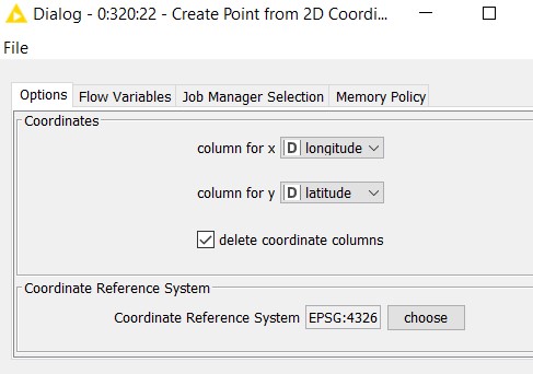
‘Create point from 2D Coordinates’ takes the two columns containing coordinates (latitude and longitude fields), and changes it into Point geometries having coordinates with the values X and Y in the Coordinate Reference System defined in the parameters.

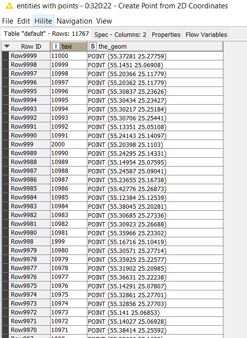
The output of the node will be as follows:

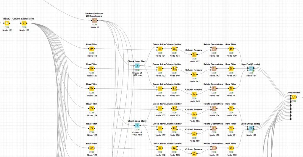
In our first approach given below, all the 11,767 taxi location records are cross joined with the 226 geo fence areas (multi-polygon geometries), and fed into one ‘Relate Geometries’ node using a Chunk loop of 1,000 rows to reduce processing overhead. Relate geometries performs operations on only two geometries at a time. Since a taxi can be present in only one geo fence area at any point of time, to find the current geo fence area of a taxi, its location must be evaluated against all 226 geo fences available. Hence a cross join is performed here.

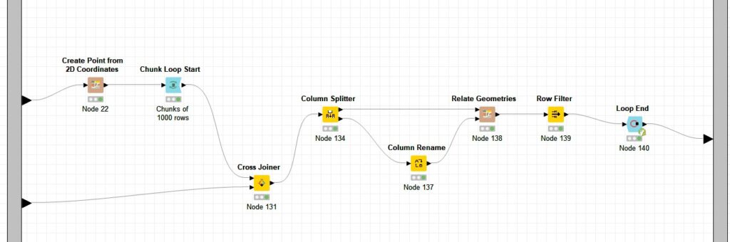
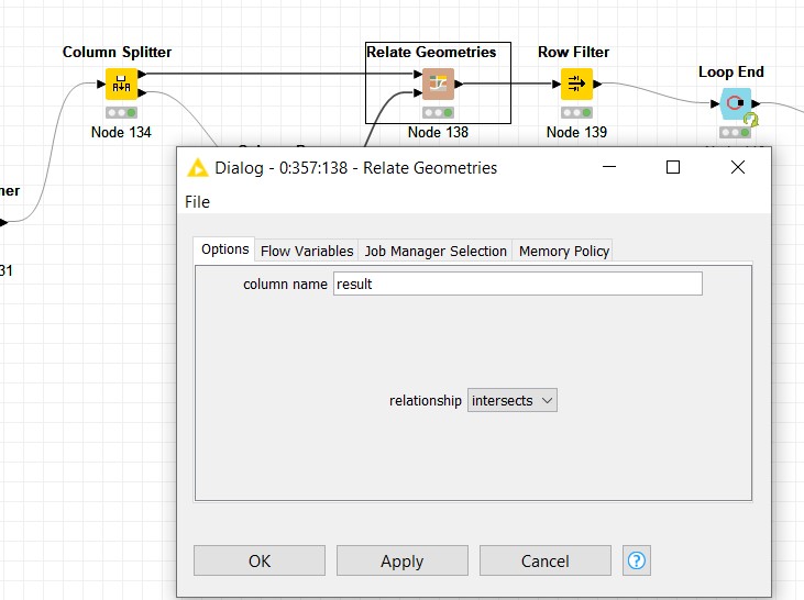
Relate Geometries takes two tables which have the same count of entities as inputs. In our example, the top partition contains the point geometries of taxi locations and the bottom partition contains the multi-polygon geometries (226 in number) which correspond to the areas.

Since we need to find the areas in which taxis are located, we selected the “intersects” relationship in the ‘Relate Geometries’ configuration.

The operator will be applied line by line the operator, and the result will be appended as a novel Boolean column of the first table. That is, if a taxi is present in a particular area, the result of the intersection operation would be true, and vice versa.

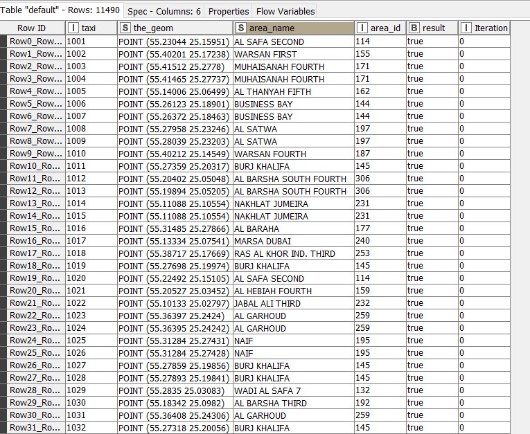
We use the row filter to display only the results having true values, which gives us 11,490 taxis and their corresponding areas. The remaining 277 taxis don’t fall in any of the 226 geo fence areas.

2. Second Approach: Using KNIME standard Spatial Processing nodes with parallel process

The earlier approach was very time consuming, resource intensive, and a sequential operation. A line by line intersection operation on 11,767 x 226 = 2,659,342 records is carried out. The approach took about 30 minutes on a personal laptop.

To parallelize this, in our second approach, we have split the area data on a key column and used multiple Relate Geometries nodes as below:

In our example, the areas were split into 18 buckets and 18 Relate Geometries were used in parallel. Then, true valued results were concatenated to produce the final output.

This approach took about 8 minutes and is four times faster than the first one, but we ended up using multiple threads in a single workflow and caused clogging of other workflows. So this is not an ideal method either.

3. Final Approach: Using Python Spatial Join (Geopandas)

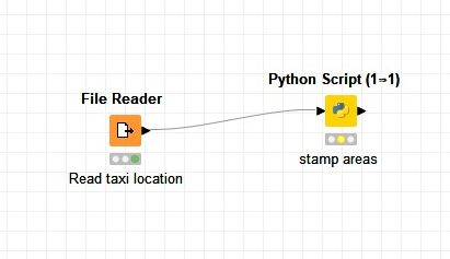
We finally arrived at an efficient approach to do a spatial join through Python script in KNIME. Our objective is still to reduce the runtime significantly, while using as few resources as possible.

A spatial join is when you append the attributes of one layer to another, based upon its spatial relationship. In our example, we need to apply the “area” attribute to every taxi that is spatially in a particular area.

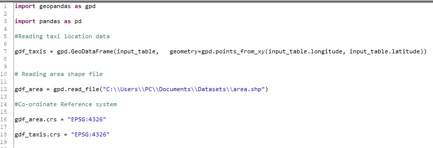
In our example, taxi data with latitude and longitude columns are the input table to the python script. The Geopandas conversion adds the geometry column, which allows us to do the spatial join. Thus, point geometries will be created for gdf_taxis. Area data (polygon geometries) are read from shape file, ‘area.shp’. Geojson files can also be directly read in a similar fashion.

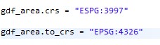
The CRS of both the data to be joined, gdf_taxis and gdf_area, should be the same. If the data corresponds to different CRS (say, area is in ‘3997’), it can be converted to the desired CRS as shown below:

To apply a join, we use geopandas.sjoin() function as below:

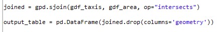
The ‘op’ argument specifies the type of join that will be applied. op = “intersects” returns true if the boundary and interior of the object intersect in any way with those of the other.

Thus, with one line of code, we can determine the taxis in each area. The output of the python script is as below:

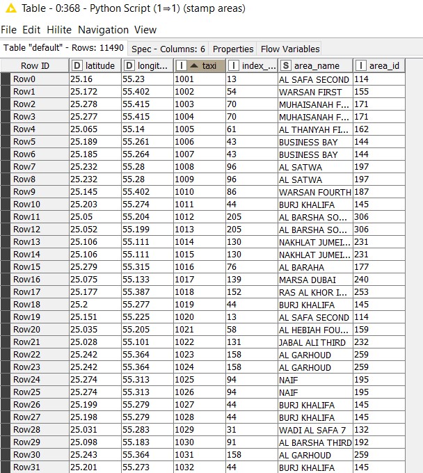
This approach took about 4 seconds to complete and is 120 times faster than the second approach, giving us great improvements in execution time and resource consumption.

Summary and Conclusion

1. The first approach of using the KNIME nodes took about 30 minutes. It was nowhere near our customer’s SLA requirements.
2. The second approach of using the KNIME nodes but with parallelization resulted in 8 minutes. Although this was ~4x better than the first, it still did not meet our customer’s SLA requirement and moreover, it was extremely resource intensive as well.
3. The final approach of using the python code snippet node resulted in a completion time of 4 seconds. This approach put us way ahead of our customer’s SLA requirements, and the resource requirements were well within limits as well.

Thus, the python and KNIME combination provided 450x performance in terms of speed compared to the standard KNIME spatial nodes. This goes to show how seamlessly KNIME’s capabilities can be enormously increased with python or other open source tools in your use cases.

Please follow this space for more interesting articles about KNIME and its applications. We’d love to help you with complex data challenges in your organization, from engineering to machine learning, with our innovative solutions. Simply drop us a note at info@clearpeaks.com or sales@clearpeaks.com.