22 Nov 2023 How to Improve Data Extraction Performance from Cloudera Data Warehouse to Load a Microsoft SSAS Tabular Model
Large company data warehouses are often made up of several platforms that are interconnected to provide a data model which allows users to work with the information they need.
This type of scenario poses significant challenges in developing a solution that is easy to maintain, while still meeting the users’ requirements.
One of these challenges is extracting data from one platform to store it in another, which raises several questions, such as:
- How can those platforms be connected?
- What connectors are available?
- How should data types be managed to avoid misinterpretation?
In this context, other challenges are:
- How can we deal with excessively long processing times with high data volumes?
- How can we avoid the maintenance of platforms that have the same information (creating unnecessary redundancies and additional storage costs)?
- What tool can we provide to users that allows them to exploit the data through a friendly model that they can easily understand (providing what has been called “self-service data analytics”)?
Based on these premises, one of the scenarios that we have faced here at ClearPeaks is how to extract data from a data warehouse based on a Cloudera platform to exploit it through a friendly tool, like an SQL Server Analysis Services (SSAS) tabular model, without duplicating the backend model in an SQL Server database engine structure.
Faced with this situation, most would be tempted to create an ETL that extracts the data from Cloudera, stores it in an SQL Server database, and then exploits it by building a tabular model in SSAS that connects to the SQL Server database, as follows:
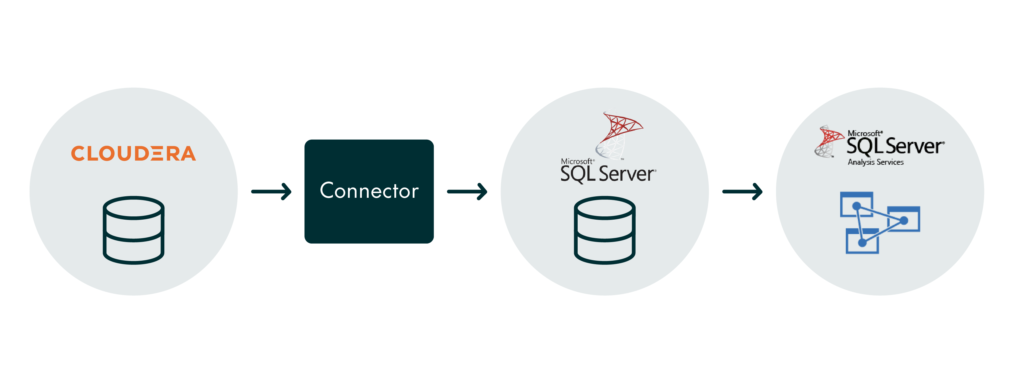
However, this approach means maintaining two data warehouses instead of just one. It implies having two backend databases, which would necessitate additional investment in storage to accommodate the duplicate data.
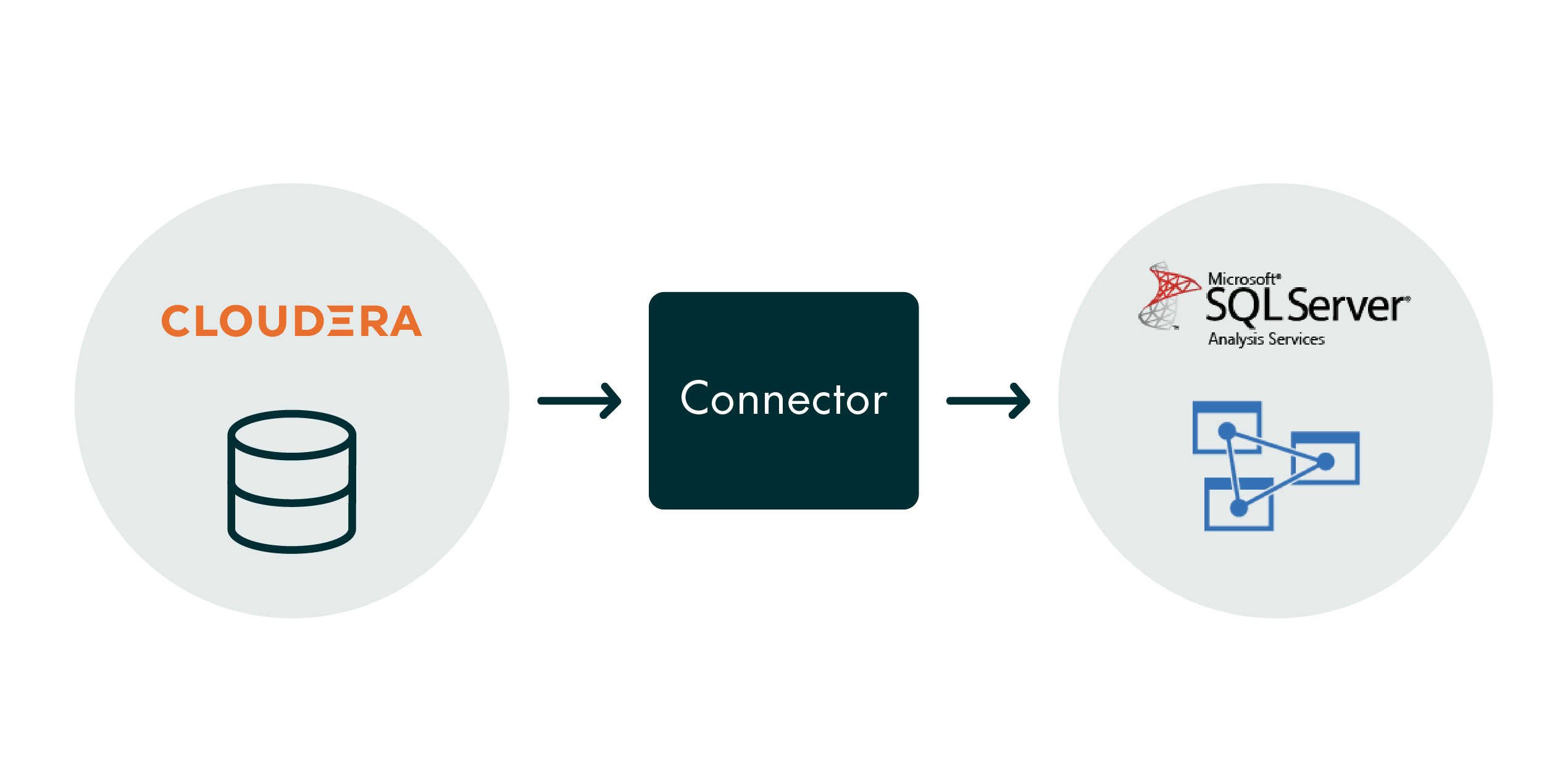
In line with this scenario, and to avoid maintaining two data warehouses, the best solution is to extract the data and insert it directly into an SSAS tabular model database, without involving an SQL Server database engine. So, the solution could be re-drawn as follows:
Connecting SSAS Tabular Model to Cloudera
The first and perhaps most critical challenge is how to connect an SQL Server Analysis Services instance with a tabular model to the Cloudera ecosystem.
One of the aspects to consider is that SSAS in tabular mode does not have a native driver to connect to Cloudera, so it is necessary to come up with an approach that allows us to read the data and load it into the SSAS database.
After analysing the alternatives available, we can focus on three options:
- Cloudera-native ODBC Driver: Installing the native Cloudera ODBC driver to connect to the data by using Impala as the SQL query engine.
- CDATA ODBC Driver: Installing the CDATA ODBC driver to connect to the data by using Impala as the SQL query engine. Note: CDATA is a vendor that provides this kind of connector to read data from different sources.
- CSV Files: Generating CSV files containing data from various tables, which are then transferred from Cloudera to the SSAS server via a mount point configured between both platforms. Subsequently, the files are loaded into the SSAS server using a data source in Text/CSV file format, which is native in SSAS tabular mode.
This revision breaks the complex process down into more digestible parts, making it clearer and easier to follow.
We were pretty excited to have more than one way to do this. However, selecting one was not as easy as we expected!
Let’s dive deep into each case:
- Cloudera-native ODBC Driver
By installing the native Cloudera ODBC driver, we could connect to the data and extract it. However, the performance for big tables (more than 1 million rows) was not what we’d hoped for. For example, it took 27 minutes to load a table that contained 1.3 million rows, which is much too long for this type of table. - CDATA ODBC Driver
The CDATA ODBC driver loaded the same data in 9 minutes, so at first glance, this seemed promising. However, the scenario changed when we attempted to load 10 tables, each with over 10 million rows. The performance was significantly impacted – it took more than 6 hours to load all the tables. This fell way short of our expectations, especially considering our Service Level Agreement (SLA) required the cube to be available within just 1 hour. - CSV Files
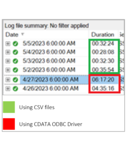
Third time lucky! We created an ETL to generate CSV files and transfer them to a mount point configured between Cloudera and the SSAS server. Performance was dramatically improved, from around 6 hours to around 40 minutes (including CSV file generation and transfer), which means a 90% improvement: Another advantage of this approach is that by using CSV files all the columns can be treated as text, simplifying data interpretation.
 Another advantage of this approach is that by using CSV files all the columns can be treated as text, simplifying data interpretation.
Based on the results above, we’ve got the following:
Approach | Number of rows | Processing time (sec.) |
|---|---|---|
| Cloudera native ODBC driver | 1,300,000 | 1620 |
| CDATA ODBC driver | 1,300,000 | 540 |
| CSV files | 1,300,000 | 54 |
However, when it came to loading small and medium-sized tables – small tables having 1 to 999 rows, and medium ones ranging from 1,000 to 999,999 rows – the performance improvement was not significant: the time taken for file generation, transfer, and final data loading remained very similar. This observation led us to conclude that a hybrid solution was necessary, so we opted to load the large tables via CSV files (gaining a 90% performance improvement) and the small and medium tables directly using the CDATA ODBC driver.
Based on the above, we now have the following setup:
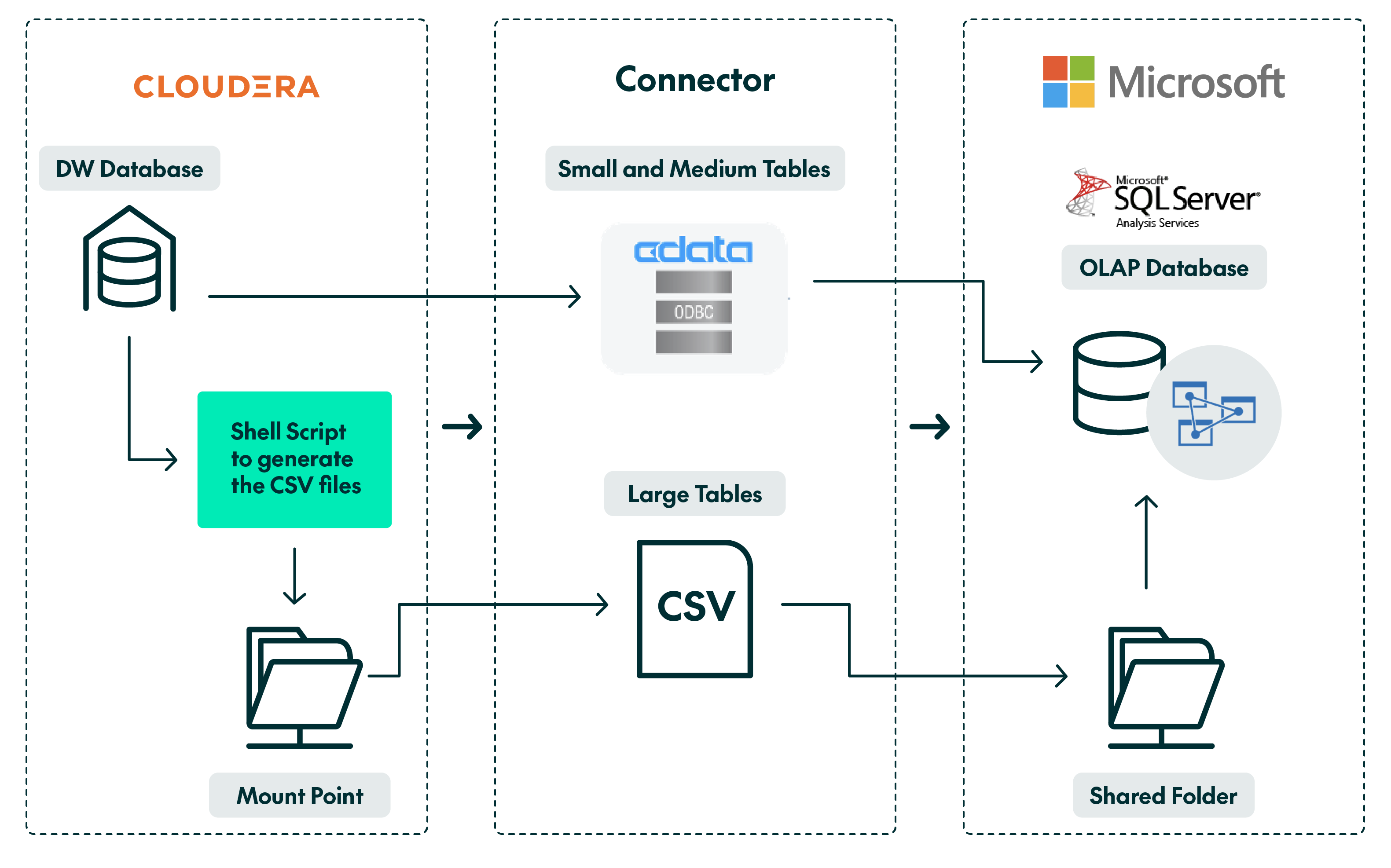
Note that the process involves two key steps: on the Cloudera side, a shell script is used to generate and store the CSV files on a mount point, while on the Windows side, an SSIS package moves these CSV files to a local path on the server. The files are then moved into the SSAS database.
SSAS Table Configuration
Having opted for a hybrid solution, our next challenge was to configure the SSAS tables so that we could load them based on their size. It is important to take into account that, due to their size, the fact tables were partitioned by month and/or year, depending on the number of rows they had.
Considering this premise, it was also important to note that the new records for the specified fact tables did not exceed 1 million rows per day, so we developed an ETL process to dynamically load the new daily rows from the fact tables, i.e., an incremental load, along with the medium and small tables during weekdays, and on weekends, data from the last two partitions of each fact table was completely reloaded using CSV files. This approach was designed to reorganise the data in its respective partitions.
In this context, the processing of these tables was set up using XMLA scripts where the M language expression used in each case was dynamically modified, as follows.
Daily Fact Table Loading
This process runs during the week, from Monday to Saturday:
{
  "sequence": {
    "maxParallelism": 3,
    "operations": [
      {
        "refresh": {
          "type": "add",
          "objects": [
            {
              "database": "SSAS database name",
              "table": " fact table name 1",
              "partition": "Partition name of the fact table 1"
            },
            {
              "database": "SSAS database name",
              "table": " fact table name 2",
              "partition": "Partition name of the fact table 2"
            },
            {
              "database": "SSAS database name",
              "table": " fact table name N",
              "partition": "Partition name of the fact table N"
            }
          ],
          "overrides": [
            {
              "partitions": [
                {
                  "originalObject": {
                    "database": " SSAS database name ",
                    "table": " fact table name 1",
                    "partition": "Partition name of the fact table 1"
                  },
                  "source": {
                    "type": "m",
                    "expression": [
                      "let",
                      "    Source = Odbc.Query(DSN, \"select * from <fact table name 1> where date between <start date/time> and <end date/time>;\")",
                      "in",
                      "    Source "
                    ]
                  }
                },
               {
                  "originalObject": {
                    "database": " SSAS database name ",
                    "table": " fact table name 2",
                    "partition": "Partition name of the fact table 2"
                  },
                  "source": {
                    "type": "m",
                    "expression": [
                      "let",
                      "    Source = Odbc.Query(DSN, \"select * from <fact table name 2> where date between <start date/time> and <end date/time>;\")",
                      "in",
                      "    Source "
                    ]
                  }
                },
               {
                  "originalObject": {
                    "database": " SSAS database name ",
                    "table": " fact table name N",
                    "partition": "Partition name of the fact table N"
                  },
                  "source": {
                    "type": "m",
                    "expression": [
                      "let",
                      "    Source = Odbc.Query(DSN, \"select * from <fact table name N> where date between <start date/time> and <end date/time>;\")",
                      "in",
                      "    Source "
                    ]
                  }
                }
              ]
            }
          ]
        }
      }
    ]
  }
}
The start date/time and the end date/time must be provided at runtime.
Weekend Fact Table Loading
This process runs on Sundays only:
{
  "sequence": {
    "maxParallelism": 3,
    "operations": [
       {
        "refresh": {
          "type": "dataOnly",
          "objects": [
            {
              "database": "SSAS database name",
              "table": " fact table name 1",
              "partition": "Partition name of fact table 1"
            },
            {
              "database": "SSAS database name",
              "table": " fact table name 2",
              "partition": "Partition name of fact table 2"
            },
            {
              "database": "SSAS database name",
              "table": " fact table name N",
              "partition": "Partition name of fact table N"
            }
          ],
          "overrides": [
            {
              "partitions": [
                {
                  "originalObject": {
                    "database": " SSAS database name ",
                    "table": " fact table name 1",
                    "partition": "Partition name of the fact table 1"
                  },
                  "source": {
                    "type": "m",
                    "expression": [
                      The “M language” script to process each CSV file to load the fact table 1.
                    ]
                  }
                },
  {
                  "originalObject": {
                    "database": " SSAS database name ",
                    "table": " fact table name 2",
                    "partition": "Partition name of the fact table 2"
                  },
                  "source": {
                    "type": "m",
                    "expression": [
                      The “M language” script to process each CSV file to load the fact table 2.
                    ]
                  }
                },
  {
                  "originalObject": {
                    "database": " SSAS database name ",
                    "table": " fact table name N",
                    "partition": "Partition name of the fact table N"
                  },
                  "source": {
                    "type": "m",
                    "expression": [
                      The “M language” script to process each CSV file to load the fact table N.
                    ]
                  }
                }
              ]
            }
          ]
        }
      }
    ]
  }
}
Note that for the above two scripts (daily and the weekend) you must set the maxParallelism parameter to 3, which means that up to three objects will be processed in parallel. This is recommended to prevent the server from crashing due to lack of memory. Needless to say, you can set another number based on your server size.
You can also add as many tables as you need in the highlighted sections, regardless of the maxParallelism value you have set. For more information about this parameter, check out this link.
Small/Medium Table Loading (Model Dimensions):
      {
        "refresh": {
          "type": "add",
          "objects": [
            {
              "database": "SSAS database name",
              "table": "table name",
            }
          ]
        }
      }
Remember that this last type of table must be configured beforehand as follows:
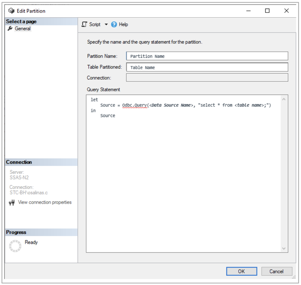
Note that the Query Statement includes an SQL query, instantiated on the server side (in this case on Cloudera), using the corresponding Data Source Name (DSN), which you will have had to configure previously on the server through the ODBC Data Source Administrator.
Logic Used to Process the Tables
At a high-level view, the ETL to process the SSAS database tables must fulfill the following logic:
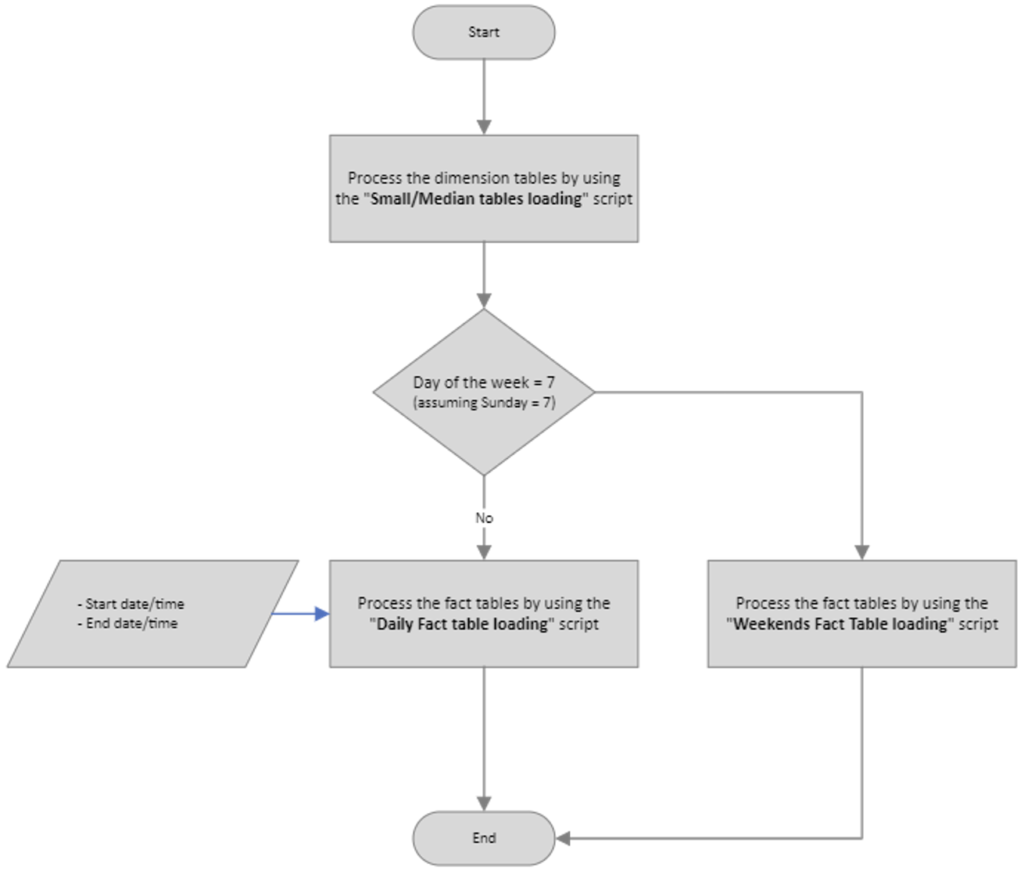
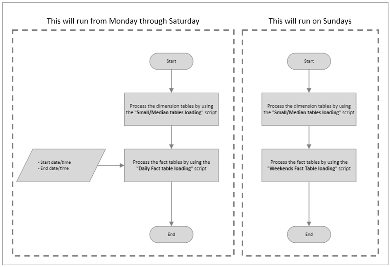
For the ETL process, input dates and times (start date/time and end date/time) must be supplied to the fact table loading (during the week) script for each fact table that needs processing. Alternatively, you might consider implementing two distinct ETL processes – one operating from Monday to Saturday and another exclusively for Sundays, as outlined below:
Remove Old Uploaded Files to Prevent Storage Filling Up
In the context of a data warehouse backend that contains historical data, there’s no need to store files for an extended period once they’ve been loaded, so it’s advisable to incorporate a task that deletes files which are already uploaded to the SSAS database and are older than a predetermined period. This approach will help to prevent the unnecessary filling up of your organisation’s storage devices.
You might ask how to determine the appropriate period for file retention before deletion: the duration for which files remain on the storage device depends on several factors which require careful analysis. To define this period, consider aspects such as the size of each file, the urgency of data restoration from a specific table under certain circumstances, and the available storage space. While there are other factors to consider, these provide a solid starting point.
In the scenario described in this article, we dealt with files of varying sizes, with the total size for each load (weekends only) being approximately 300 GB. Considering the available disk space of 6TB, and setting a conservative allocation of 20% for CSV file data, we determined that retaining one month’s worth of files was optimal:
Used Space (GB) = 300 GB x 4 weeks = 1,200 GB per month
Used Space (TB) = 1,200/1,024 = 1,17 TB
% Space = 1,17 / 6 à 20% of used space
As a result, the ETL that runs on weekends also deletes files a month after they were uploaded.
Additionally, considering the time it takes to generate CSV files – approximately 10 minutes per file – we found it unnecessary to keep more than this number of files readily available. This approach can handle any special situations that might occur, without unnecessarily occupying storage space.
Conclusions
In this article, we’ve explored various methods, both individually and in combination, for utilising SSAS to analyse data from Cloudera Data Warehouse, focusing particularly on the size of the source tables. Our experience confirms that for tables exceeding 1 million rows, loading data via CSV files is highly advantageous, offering significantly better performance than using ODBC drivers (including the native Cloudera driver or others).
However, to expedite development times and avoid the need to create specific routines for generating CSV files for each table in your SSAS data model, ODBC drivers are a viable option for medium and small tables, given the comparable performance.
In our scenario, we adopted a hybrid approach, leveraging the strengths of both CSV file loading and ODBC drivers; this approach maximised efficiency and performance. It’s also important to free up storage space after loading CSV files to prevent unnecessary clutter.
Considering all this, our recommendation is to thoroughly test the processing performance of your SSAS tabular model, finding your comfort zone whilst ensuring you meet the solution’s availability requirements.
If you need more details about this solution and how to adapt it to your needs, or if you have any questions about how to harness the power of Cloudera for your organisation, please contact us here at ClearPeaks and we will be glad to assist you!