08 Nov 2023 Introduction to Apache Iceberg

Apache Iceberg is an open-source data table format originally developed at Netflix to overcome challenges faced by existing data lake formats like Apache Hive. Boasting capabilities such as support for ACID transactions, time-travel, in-place schema, partition evolution, data versioning, incremental processing, etc., it offers a fresh perspective on open data lakes, enabling fast and efficient data management for large analytics workloads.

Thanks to all this, and especially thanks to its ability to handle partitions and data changes so well, Iceberg is becoming more and more popular, now adopted by many of the top data platform technologies such as Cloudera, Snowflake, Dremio, and so on.

In this blog post, we will provide a hands-on introduction to the tool, delving deep into some of its fundamental functionalities and looking at the benefits it offers, using a local instance based on the open-source version to do so.

Why Use Apache Iceberg?

Apache Iceberg was primarily designed to effectively address the limitations encountered with Apache Hive, particularly the numerous design challenges faced when operating at scale with extensive datasets. For example:

• The performance issues when fetching the (complete) directory listings for large tables.
• The potential data loss or inconsistent query results after concurrent writes.
• The risk of having to completely rewrite partitions after updates or deletions.
• The need to re-map tables to new locations after modifying existing partitions, due to the fixed definition of partitions at table creation, making modifications impractical as the tables grow.

Apache Iceberg addresses these problems by combining the benefits of both traditional data warehousing and modern big data processing frameworks. Thanks to its innovative table data structure, the efficient use of metadata files to track changes, and the optimal use of indexes, Iceberg can offer much better performance, whilst also introducing many new features, some of which we will run through later on in the hands-on section.

Iceberg Architecture

But how does Iceberg do all of this? Mainly, thanks to its innovative architecture, built upon three distinct layers: the Iceberg Catalog, the Metadata Layer, and the Data Layer.

Iceberg Catalog

The Iceberg Catalog Layer contains the location of the current metadata pointers. Pointers pinpoint the precise location of the metadata file for each table, effectively telling any query engine (Iceberg, Spark, Hive, etc.) where to read or write data. The catalogue can be the built-in Iceberg Catalog, or others like Hive Metastore, Apache Hudi, etc.

Metadata Layer

The Metadata Layer is responsible for managing the metadata associated with Iceberg tables. It provides information about the table schema, partitioning scheme, file locations, statistics, and other properties. It consists of the following components, organised in a logical hierarchy:

1. Metadata file: This stores the schema, partition information, and snapshots, which are objects pointing to a version of the table at a given point in time. Whenever a change is made to an Iceberg table, a new snapshot is created and the “current snapshot” pointer is updated.
2. Manifest list: This contains a list of manifest files that make up the snapshot, as well as information about their location and corresponding partitions.
3. Manifest files: To track data files and provide additional information about them, like file format, scan planning, partitioning, pruning, and column level stats such as min/max values. Iceberg takes advantage of the rich metadata it captured at write time and leverages the aforementioned techniques for enhanced performance.

Data Layer

The Data Layer is, quite obviously, where the data is stored, and it can reside in HDFS, AWS S3 or Azure Blob Storage. It consists of data files containing actual records in columnar format (like Parquet or ORC), organised in partitioned directories. Data files also contain some additional information, such as partition membership, row count, and upper and lower bounds.

Layer Interaction

Now that we know the purpose of each layer, let’s look at an example of how they behave and interact with each other.

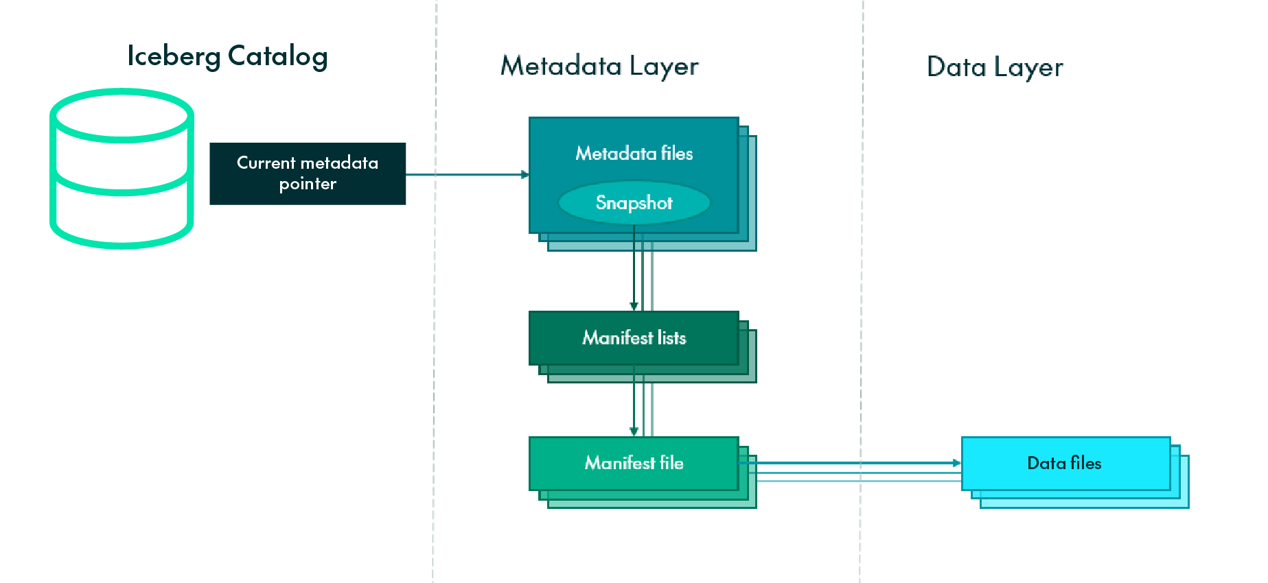
Figure 1: Iceberg architecture layers.

When a SELECT query is executed on an Iceberg table, the query engine first consults the Iceberg Catalog, which retrieves the entry containing the location of the current metadata file associated with the target table.

The query engine then moves from the Iceberg Catalog to the Metadata Layer, and proceeds to open that metadata file, reading the value of the current-snapshot-id, getting the location of the corresponding manifest list, then reading the manifest-path entries and opening the associated manifest files, which contain the path to the actual data files.

At this stage, the engine may optimise operations by utilising row counts or applying data filtering based on partition or column statistics, which are already available in the manifest files. If required, the query engine finally goes into the data layer, fetching the corresponding data files.

Hands-on

Setting Up the Environment

Now that we have introduced the “theory” behind Iceberg, let’s do some hands-on testing of its most interesting features. In this blog post we will cover the following: in-place schema evolution, partition evolution, time-travel and rollback.

To do so, we used a ready-to-use Docker image to set up a quick Iceberg instance running on Spark 3 (follow this link from Dremio if you want to try the same setup). Please note that the environment setup and subsequent table creation described here are for demonstration or testing purposes and may vary depending on your specific requirements and configurations.

Once done, we can initialise a very user-friendly spark-sql shell with the following command:

iceberg-init

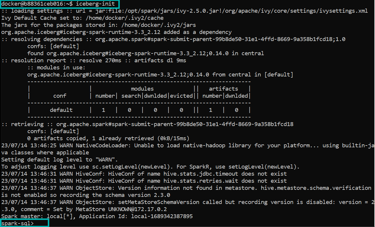
Figure 2: Ready-to-use SQL shell.

Now we are ready to test Iceberg. First of all, we’ll define a sample table to use during our tests, so we’ll create a table named “products” with information about some products and their reviews, using nested data types (follow this link to see more details on Iceberg data types):

CREATE TABLE iceberg.db1.products (
	product_id int, 
	info struct<name string, price decimal(3,2)>, 
	discounts array<float>, , 
	feedback map<string, struct<comment string, rating int>>)
USING ICEBERG;

As explained above, this command generates an entry in the Iceberg Catalog for the created table (stored as version-hint.text) pointing to the newest metadata file (as it is the first version of the table, this file is named v1.metadata.json). We can check this by navigating to it through the file system as shown below:

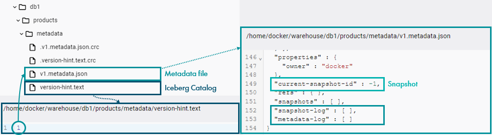
Figure 3: Create table metadata files.

Now, let’s see how these metadata files are updated when we ingest some data into the table:

INSERT INTO iceberg.db1.products VALUES 
	(1, 
	struct("product 1", 1), 
	array(5.5, 10), 
	map("customer 1", struct("Perfect", 5)));

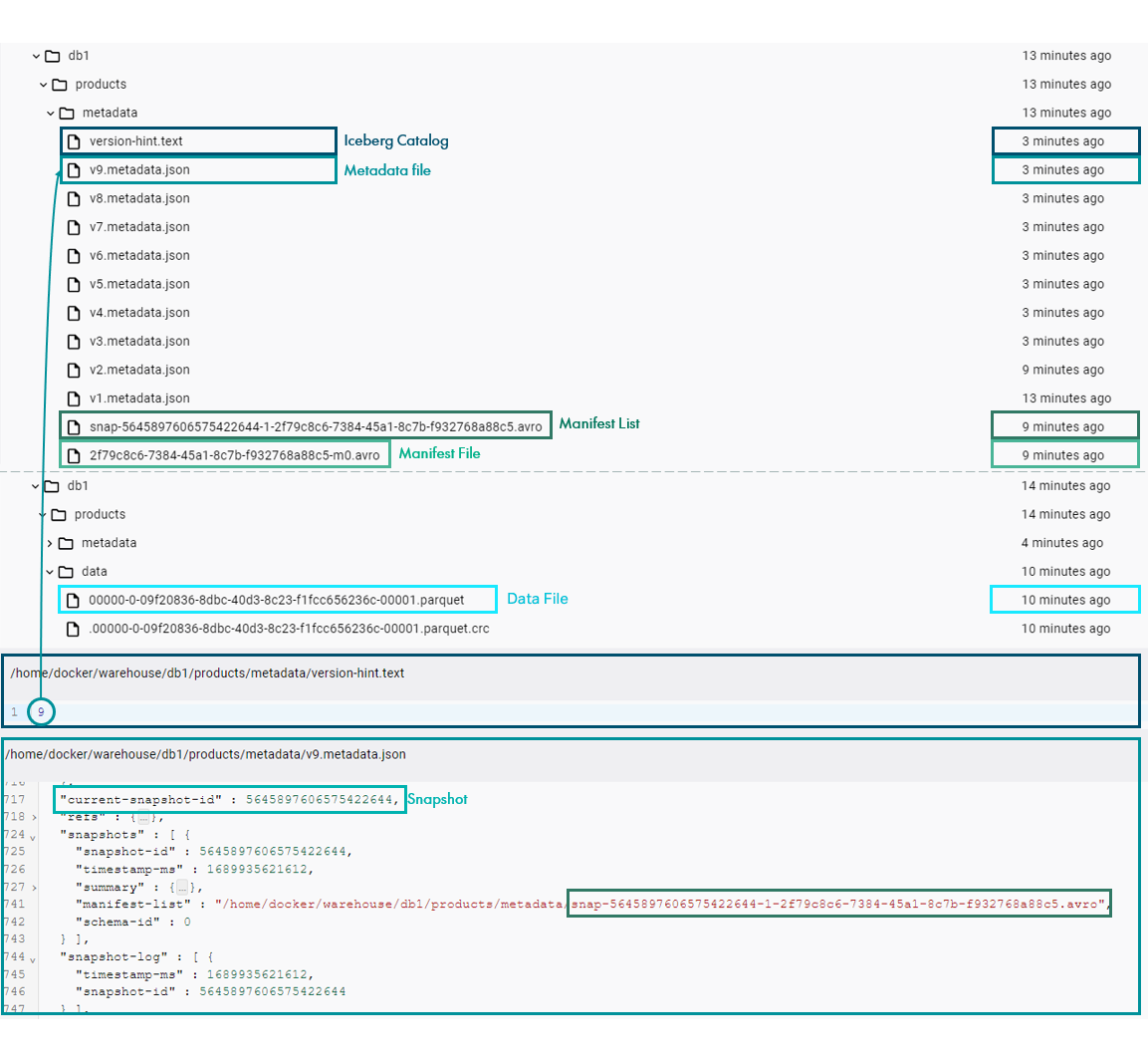
We can see that the table contains a new folder called data, representing the data layer, where we can now find a Parquet file containing the new ingested record. We can also see that the following files were generated in the metadata layer: a manifest file (XXX.avro) pointing to the mentioned data file, a new manifest list (snap-ID-XXX.avro) referring to this manifest, and a new version v2 of the metadata file, pointing to the snapshot. Finally, we can see that the Iceberg Catalog has been updated with the newest version number:

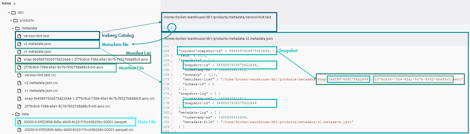
Figure 4: Metadata files after Insert.

If we now execute a select statement to read the table, the query engine will go through the following steps:

SELECT * FROM iceberg.db1.products;

Figure 5: Select table output.

1. The query engine accesses the Iceberg Catalog: version-hint.text.
2. The Iceberg Catalog retrieves the current metadata file location entry: 2.
3. The metadata file metadata.json is opened.
4. The entry for the manifest list location for the current snapshot is retrieved: snap-ID-XXX.avro.
5. The manifest list is then opened, providing the location of the manifest file: avro.
6. The manifest file is opened, revealing the location of the data file: data/YYY.parquet.
7. This data file is read, and as it is a SELECT * statement, the retrieved data is returned to the client.

Now that our table is ready, we can start testing Iceberg’s latest functionalities.

Schema Evolution

The schema of an Iceberg table is a list of columns defined in the metadata file. Their details are stored in a struct type, containing their corresponding name and a unique identifier in the table. To maintain consistency, Iceberg columns are ID-based instead of name-based, enabling safe schema evolution, as the columns have a static ID, unlike names that can be changed or reused.

When the schema of an Iceberg table is changed, a new metadata.json file is generated, containing the new definition. The changes occur only at metadata level: the existing data files are not altered! In other words, schema changes do not create a new snapshot, and so historical data remains accessible and unaffected.

Iceberg allows both primitive and nested data types, like Struct, List, and Map, and supports the common schema evolution changes, applicable to both table columns and nested struct fields: Add, Drop, Rename, Update, and Reorder.

Whatever the applied change, Iceberg guarantees correctness, but at a cost: for example, we can’t create a new column using existing values, and neither can we drop columns that have been part of the partition tree (more details on this in the following section).

Now let’s have a look at how in-place schema evolution actually works:

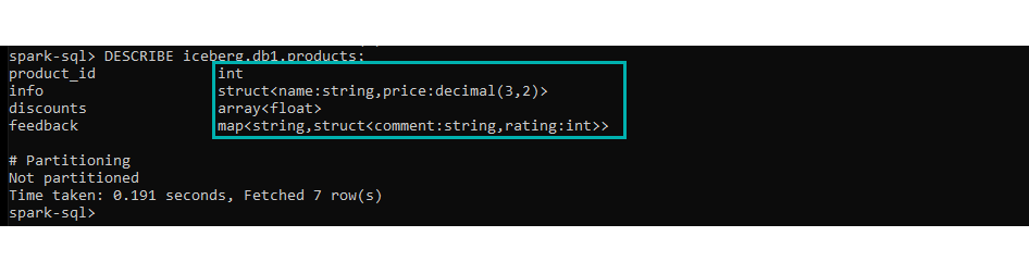
1. First of all, we’ll review the status of our table:

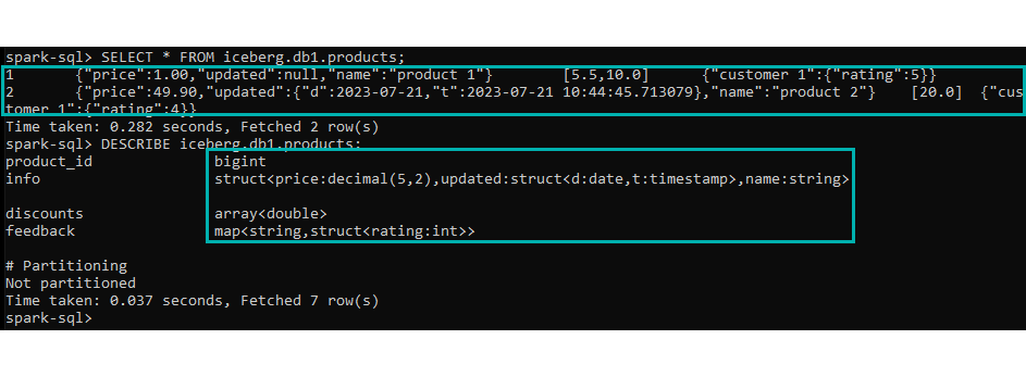
   DESCRIBE iceberg.db1.products;
   

   

   Figure 6: Schema evolution example: nested data types and current status.

   We can see that we have three nested data types. Moreover, the map field’s value contains a struct which is a nested data type. Remember that we are currently at version 2 and that there is only a single data file.

2. Now let’s make some changes to the columns:

   ALTER TABLE iceberg.db1.products ADD COLUMNS info.last_updated struct<d date, t timestamp>;
   ALTER TABLE iceberg.db1.products ALTER COLUMN product_id TYPE bigint;
   ALTER TABLE iceberg.db1.products ALTER COLUMN info.price TYPE decimal(5,2);
   ALTER TABLE iceberg.db1.products ALTER COLUMN discounts.element TYPE double; 
   ALTER TABLE iceberg.db1.products RENAME COLUMN info.last_updated TO updated;
   ALTER TABLE iceberg.db1.products ALTER COLUMN info.name AFTER updated; 
   ALTER TABLE iceberg.db1.products DROP COLUMN feedback.value.comment;
   

   In the figure below, we can see how these changes to the schema definition affected the underlying metadata. Note that the last modified time of the data file, the manifest file and the manifest list have not been changed, and the latest version of the metadata is pointing to the same snapshot as before:
   

   Figure 7: Schema evolution metadata changes.

3. Now we’ll add some more data, following the new table format:

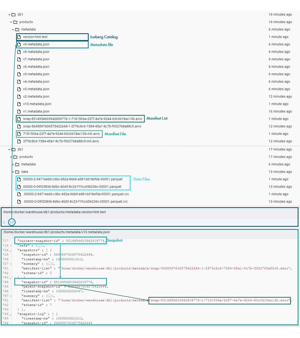
   INSERT INTO iceberg.db1.products VALUES
   	(2,
   	struct(49.9, struct(date(now()), timestamp(now())), "product 2"),
   	array(20),
   	map("customer 1", struct(4)));

   We can see that despite the changes to the schema, new data was ingested to the table as normal. If we look at the associated files, the Iceberg Catalog is now pointing to a new version of the metadata, which was generated based on the previous metadata file while updating the pointer to the new snapshot ID.

   We can also see that a new snapshot and its corresponding manifest list and files have been created to incorporate the recently ingested data location and statistics. Finally, we can see that a new data file has been added to the data layer as well:
   

   Figure 8: Schema evolution metadata changes.

    

   Note that all of these files are processed, from the most specific (Data Layer) to the least (Iceberg Catalog) for two different reasons. Firstly, the upper metadata needs to know the location of its pointed files, so they need to exist before. Secondly, to maintain consistency: if any reader tries to access the data while these steps are in progress, they would keep reading the previous value of the Iceberg Catalog, reading all the metadata and data associated with the table prior to any of the changes.

4. Finally, let’s check the new status of our table:

   SELECT * FROM iceberg.db1.products; 
   DESCRIBE iceberg.db1.products;
   

   

   Figure 9: Schema evolution example: old vs new schema.

   Note how both the original record and the new one are correctly displayed, regardless of their underlying schema difference! As we mentioned, table changes are made efficiently and guarantee consistency and correctness.

Partition Evolution

Partitioning is a common technique to speed up a query, dividing the table into separated segments that can be quickly written and read together. Whilst this process is efficient and sometimes even necessary, setting up and maintaining a partition structure can be a very tedious task in popular table formats like Hive, and trying to change it is even more so.

In Iceberg, partitioning is hidden, and mostly transparent for users: unnecessary partitions are filtered automatically, and can evolve as required.

When querying a partitioned table, Iceberg takes advantage of the layered architecture we saw earlier, which enables both metadata filtering and data filtering. Metadata filtering is applied by filtering files using the partition value range in the manifest list, without reading all the manifest files. Data filtering is applied when reading manifest files using partition data and column-level stats, before reading the actual data files.

Iceberg’s partitioning technique offers performance advantages over conventional partitioning, as it supports in-place partition evolution, avoiding the need to rewrite an entire table. This is possible thanks to the partition-spec, which defines how to generate the partition values from a record. The partition-spec of a table is a tuple containing the following values:

• A source column id from the table’s schema; this column must be a primitive type and cannot be contained in a map or list (it may be nested in a struct).
• A partition field id to identify a partition field, unique within a partition spec.
• A transformation applied to the source column to produce a partition value.
• A partition name.

Modifying a partition simply means modifying the partition-spec of the table. This is a metadata operation and does not change any of the existing data files: new data will be written using the new partitioning scheme, but existing data will maintain the old layout, pretty much like what we saw when changing a schema.

A detailed list of the possible transformations to be applied to a partition is available here. Now we’ll test some of them, but first we need to drop the array and map columns from the “products” table, as the only nested data type supporting partitioning is the struct:

ALTER TABLE iceberg.db1.products DROP COLUMN feedback, discounts;

Bucket

Let’s start with bucketing:

bucket(n, column)

This transformation hashes the column value and then applies the module of the specified n number. It is useful for partitioning the table by columns with very different values or ones that cannot easily be classified, and another key point is that it ensures the maximum number of partitions (buckets) whilst balancing the amounts of data per bucket.

Let’s have a look at it in practice: for better visibility, we will add another identity partition to the same column so that we can easily see how the values are distributed amongst the buckets:

ALTER TABLE iceberg.db1.products ADD PARTITION FIELD bucket(2, info.name);
ALTER TABLE iceberg.db1.products ADD PARTITION FIELD info.name;

We can see that the partitions have been created correctly by executing the command below, or by navigating to the newest metadata file and checking the partition-spec property:

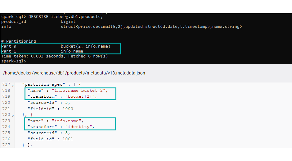
Figure 10: Bucket partition creation check.

Once our partitions have been defined, we add some more data to the table:

INSERT INTO iceberg.db1.products VALUES 
	(3, struct(20, struct(date(now()), timestamp(now())), "product 3")),
	(4, struct(15.99, struct(date(now()), timestamp(now())), "product 4")),
	(5, struct(4.49, struct(date(now()), timestamp(now())), "product 5")),
	(6, struct(20, struct(date(now()), timestamp(now())), "product 6"));

If we now check the table in the file system, we will see that two new folders have been created under the data layer, at the same level as the already existing data files. These folders correspond to the two bucket partitions we defined. If we expand them, we will find the second layer of the partition hierarchy (the identity layer), where we can see the real values of the info.name column distributed amongst the buckets:

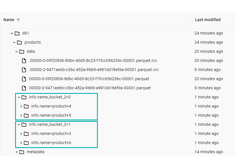
Figure 11: Bucket partition folders in data layer.

Before moving to the next partition transformation, we drop the already existing partitions so that it is easier to navigate through the folders later:

ALTER TABLE iceberg.db1.products DROP PARTITION FIELD bucket(2, info.name);
ALTER TABLE iceberg.db1.products DROP PARTITION FIELD info.name;

Deleted Partitions

Now, a technical – yet useful – note: after executing these commands, the already existing data will be kept in the same partition scheme as when it was ingested. Moreover, in Iceberg v1, partition columns are appended to the partition-spec, which enables partition addition but not deletion. In other words, even if a column is deleted from the partitions (it is no longer used to partition data), it will not be removed from the partition-spec. We can check this by executing the command below or by navigating to the latest metadata file:

DESCRIBE EXTENDED iceberg.db1.products;

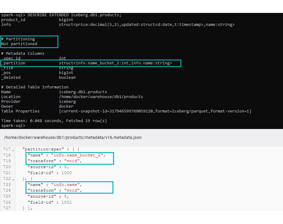
Figure 12: Describe extended partition-spec.

Here we can see that the Partitioning section in the Describe output says that the table is not partitioned. However, when checking the Metadata Columns or the metadata file, we can see that the partition-spec actually contains the already deleted partitions. From this point onward, when new data is ingested into the table, it will be stored using the null value of the deleted partitions.

Truncate

Let’s now look at truncation:

truncate(w, column)

This operation basically truncates the entry value to width w and can only be applied to string columns or numerical columns with a fixed floating point (int, long, and decimal). In the case of string, the resulting partition corresponds to the substring of the first w characters. With numerical values, a module-based formula is applied, where v is the original value: v – (v % w). Here are some examples:

For optimal visibility we will create two truncate partitions of the same decimal column, with two different widths, with w1 > w2. To facilitate the reading, we will use exponents of 10 so that when the module is applied, the remaining value corresponds to the initial digits of the original value. Additionally, we will also create a third truncate partition on column “product_id”, which is a whole number. For this partition transformation, we will use a different width to get some more complex examples:

ALTER TABLE iceberg.db1.products ADD PARTITION FIELD truncate(1000, info.price);
ALTER TABLE iceberg.db1.products ADD PARTITION FIELD truncate(10, info.price); 
ALTER TABLE iceberg.db1.products ADD PARTITION FIELD truncate(2, product_id);

In our example table, the column price is type decimal(5,2) which means that it has two decimal places, so when applying truncate(1000) the applied module is on W = 10.00, the column is truncated to tens. Similarly, when applying truncate(10), W = 0.10, the column is truncated to the first decimal place. For the last partition, the %2 will be considered. We can check this by ingesting some sample data:

INSERT INTO iceberg.db1.products VALUES 
	(7, struct(2.5, struct(date(now()), timestamp(now())), "product 7")),
	(8, struct(0.99, struct(date(now()), timestamp(now())), "product 8")),
	(9, struct(125.99, struct(date(now()), timestamp(now())), "product 9")),
	(10, struct(12, struct(date(now()), timestamp(now())), "product 10"));

To see how the data was ingested, we will navigate through the folders in the data layer (remember that new data is under the null level from the previously deleted partition).

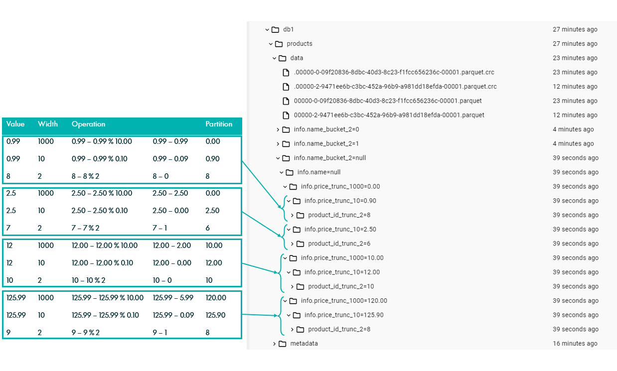
Figure 13: Truncate partition example.

Now we can move on to the last type of partition transformation. Once again, we drop the partition fields created up to this point:

ALTER TABLE iceberg.db1.products DROP PARTITION FIELD truncate(1000, info.price);
ALTER TABLE iceberg.db1.products DROP PARTITION FIELD truncate(10, info.price);
ALTER TABLE iceberg.db1.products DROP PARTITION FIELD truncate(2, product_id);

Date

We now look at date transformations, one of the most common partitioning techniques. This category includes all the possible operations that Iceberg can perform to shorten dates or timestamps: year(column), month(column), day(column) and hour(column).

Let´s test this by adding two partitions based on years and hours and one based on the identity, and then we add some sample data to our table:

ALTER TABLE iceberg.db1.products ADD PARTITION FIELD years(info.updated.d);
ALTER TABLE iceberg.db1.products ADD PARTITION FIELD hours(info.updated.t);
ALTER TABLE iceberg.db1.products ADD PARTITION FIELD info.updated.t;
INSERT INTO iceberg.db1.products VALUES 
	(11, struct(0.99, struct(date("2020-08-01"), null), "product 11")), 
	(12, struct(2.5, struct(date(now()), timestamp("2023-01-01 01:25:30")), "product 12")),
	(13, struct(2.5, struct(date(now()), timestamp("2023-07-01 11:25:30")), "product 13")), 
	(14, struct(0.99, struct(date(now()), timestamp(now())), "product 14"));

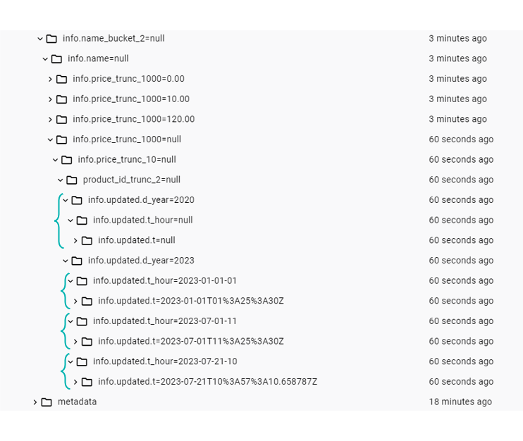
Figure 14: Date partition examples.

As we can see, timestamps and dates are correctly distributed down the partition tree, with null labels being used where the field did not contain hourly information.

A Few Comments

Thanks to all these examples of partition evolution, we have seen how modifying the partition-spec is very simple and effective. However, it is important to remember that partitions should not be modified forever, as new partitions are appended to the end of the existing partition-spec.

For our tests, we used Iceberg v1, which does not offer any simple, quick commands to solve this problem. However, Iceberg v2 introduces some new features to help overcome this drawback (you can find more details on the differences between Iceberg versions at this link).

To conclude this section, we’ll execute the following command:

TRUNCATE TABLE iceberg.db1.products;

This command deletes all the data from our table. However, if we check the data layer, we can actually still find all the data files, stored with the same partition hierarchy as before:

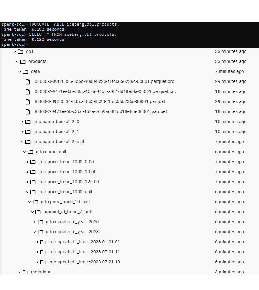
Figure 15: Truncate results.

Bearing all this in mind, we can now introduce one of the most useful features of Iceberg!

Time-travel

One of the most notable features of Apache Iceberg is time-travel, i.e. the ability to track table versions over time. As we saw, each write operation performed on an Iceberg table generates a new snapshot or version. Thanks to this, Iceberg enables us to review the snapshots captured at different points in time by navigating through the various versions of a table’s metadata.

With the history command, we can get a summary of all the versions of a given table and their respective timestamps:

SELECT * FROM iceberg.db1.products.history;

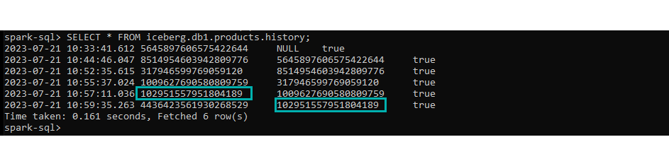
Figure 16: History of snapshots.

A similar output would be produced by the snapshots command, with the addition of the operation that generated the change, the location of the corresponding manifest list, the amount of data files that were affected, and some table statistics:

SELECT * FROM iceberg.db1.products.snapshots;

By using the information about the timestamps that we just saw, we can see the content of the table at a specific point in time by executing any of the commands below:

SELECT * FROM iceberg.db1.products TIMESTAMP AS OF ‘<timestamp>’;
SELECT * FROM iceberg.db1.products VERSION AS OF ‘<timestamp>’;

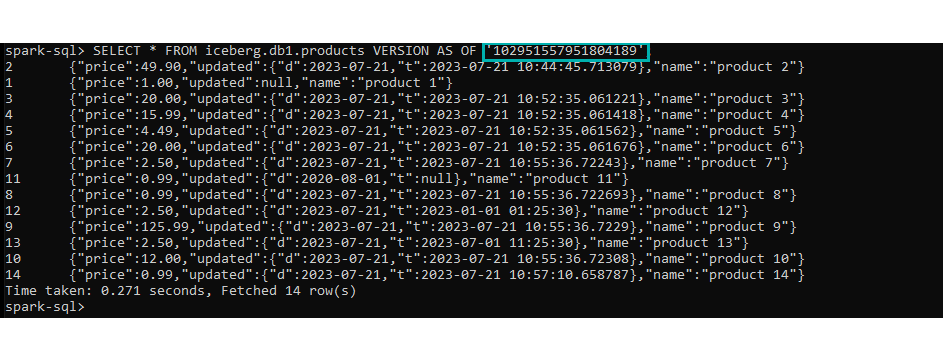
Figure 17: Query old snapshot.

When these time-travel statements are executed, the query engine will use the location of the manifest list associated with the given snapshot and proceed to read the manifest files and the corresponding data files (skipping the Iceberg Catalog and the metadata file). This means that the query will retrieve the data using the table format defined for that specific snapshot, even if the schema was altered afterwards.

We can check this by selecting the data from our first version of the table:

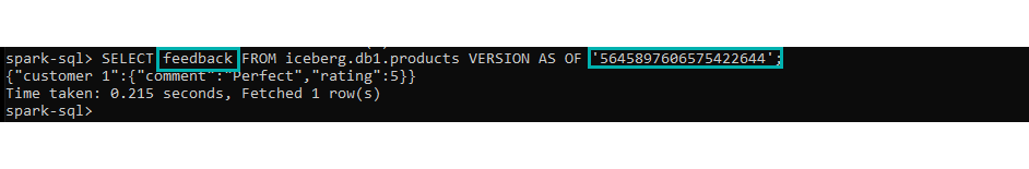
Figure 18: Query old snapshot with different schema.

Rollback

Thanks to its time-travel capabilities, Iceberg offers another exceptional feature: the rollback of a table to a previous snapshot. This is especially useful when there are accidental deletions or updates.

We use the following command:

CALL iceberg.system.rollback_to_snapshot('iceberg.db1.products', <snapshot_id> );

After the rollback, the output in the command line will display the “source“ snapshot ID (an empty truncated table) and the “destination” snapshot ID (a table filled with data), providing confirmation of the rollback process.

If we check the table history again, we will see that our “destination” snapshot appears twice: the original entry, and a new rolled-back one. Note that the “removed” snapshot is now flagged as false:

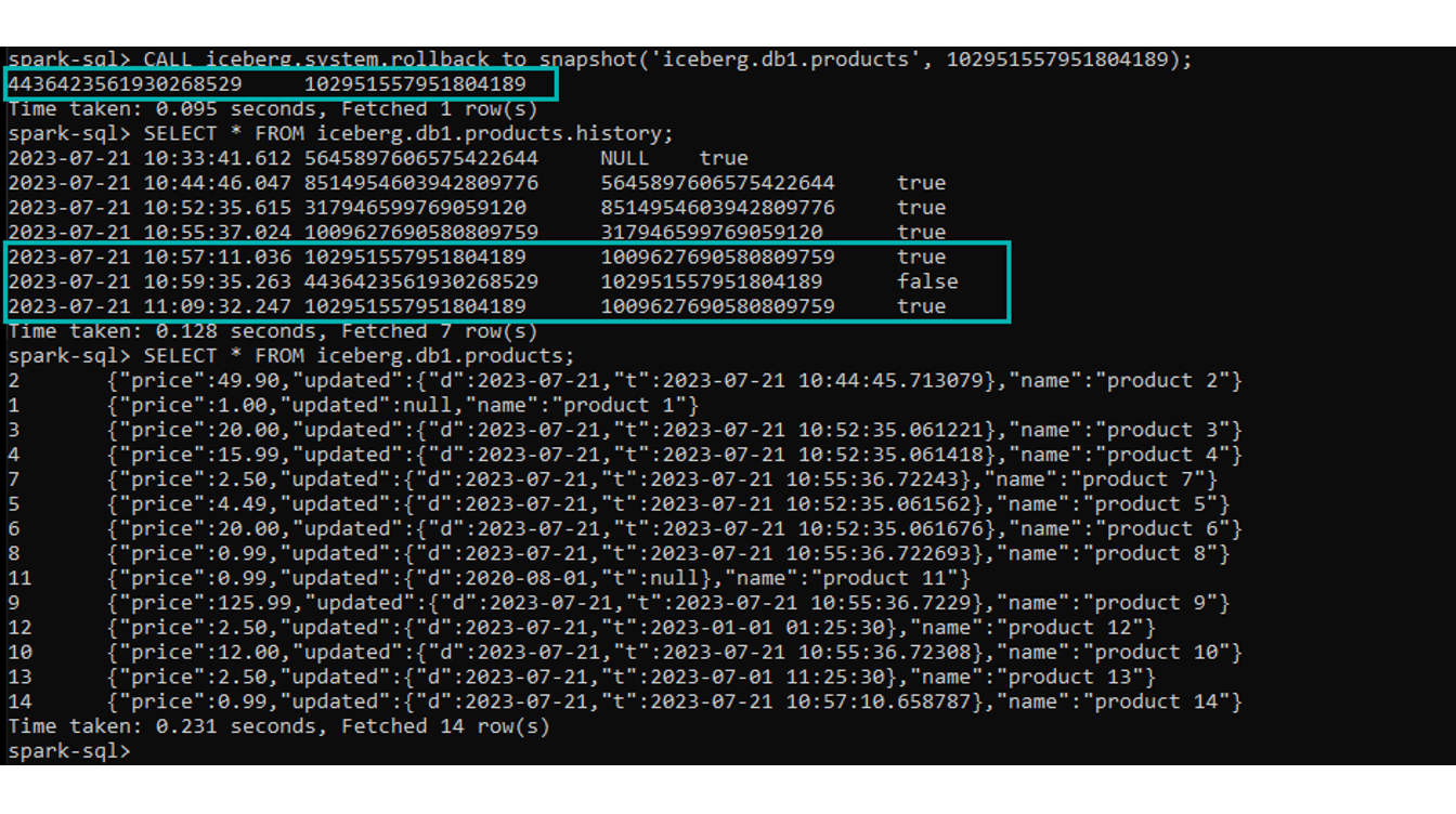
Figure 19: Snapshot history after rollback.

Remove Snapshot

As each write operation over an Iceberg table generates a new snapshot or version, the associated metadata files that you need to maintain will keep growing and growing over time. In order to reduce the size of the table’s metadata, it is recommended to regularly expire snapshots, eliminating unnecessary data files.

Iceberg offers a few ways to handle this: by default, snapshots can be automatically expired thanks to a property named “max-snapshot-age-ms”, which allows us to remove outdated snapshots based on their age (see more details on how snapshots are automatically expired at this link). Alternatively, snapshots can be removed manually, using the following command:

CALL iceberg.system.expire_snapshots('iceberg.db1.products', <timestamp>);

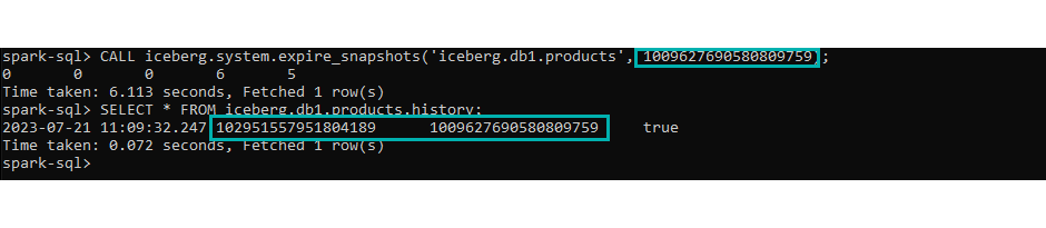
Figure 20: Expire snapshots.

Note that this command expires ALL snapshots preceding that timestamp; more details about this procedure can be found here.

Conclusion

With open data lakehouses and data mesh becoming more and more popular (check out our article here if you want to read up on this), the demand for a modern, efficient and flexible data architecture is on the rise. In this context, Apache Iceberg emerges as a cutting-edge open table format that offers distinct advantages over its historical predecessor, Apache Hive. It is no surprise that it is becoming more and more common, and it has already been adopted as a fundamental layer by many of the modern data lakehouse technologies, like Dremio, Snowflake, Cloudera, and others.

If you want to know more about Iceberg or if you are interested in embarking on the development of modern data lakehouses with the guidance of our team of experts, don’t hesitate to contact us. Our experienced professionals are ready to assist you in seamlessly setting up your environment and ensuring a smooth transition to Iceberg technology. In the meantime, stay tuned for our next blog posts, where we will bring you the practical knowledge and best practices to unlock the true potential of Iceberg for your organisation.