22 Dec 2021 Data Lake Querying in AWS – Databricks

This is the fifth article in the ‘Data Lake Querying in AWS’ blog series, in which we introduce different technologies to query data lakes in AWS, i.e. in S3. In the first article of the series, we discussed how to optimise data lakes by using proper file formats (Apache Parquet) and other optimisation mechanisms (partitioning); we also introduced the concept of the data lakehouse. We demonstrated a couple of ways to convert raw datasets, which usually come in CSV, into partitioned Parquet files with Athena and Glue. In that example, we used a dataset from the popular TPC-H benchmark, from which we generated three versions of the dataset:

• Raw (CSV): 100 GB, the largest tables are lineitem with 76GB and orders with 16GB, split into 80 files.
• Parquets without partitions: 31.5 GB, the largest tables are lineitem with 21GB and orders with 4.5GB, also split into 80 files.
• Partitioned Parquets: 32.5 GB, the largest tables, which are partitioned, are lineitem with 21.5GB and orders with 5GB, with one partition per day; each partition has one file and there around 2,000 partitions for each table. The rest of the tables are left unpartitioned.

Starting with that first blog, we have been showing different technologies to query data in S3. In the second article we ran queries (also defined by the TPC-H benchmark) with Athena and compared the performance depending on the dataset characteristics. As expected, the best performance was observed with Parquet files. However, we determined that for some situations, a pure data lake querying engine like Athena may not be the best choice, so in the third article we introduced Redshift as an alternative for situations in which Athena is not recommended. As we discussed in that blog, Amazon Redshift is a highly scalable AWS data warehouse with its own data structure that optimises queries; and in combination S3 and Athena it can be used to build a data lakehouse in AWS. Nonetheless, there are many data warehouses and data lakehouses in the market with their own pros and cons, and depending on your requirements there may be other more suitable technologies.

In the fourth article of this series we introduced Snowflake, an excellent data warehouse that can save on costs and optimises the resources assigned to our workloads, going beyond data warehousing since it can also tackle data lakehouse scenarios in which the data lake and the transformation engine are provided by the same technology.

In this article, we will look at Databricks, another data lakehouse technology that is widely used to work on top on existing data lakes. We have already talked about Databricks in past blogs like in: Mapping Data Flows in Azure Data Factory, Cloud Analytics on Azure: Databricks vs HDInsight vs Data Lake Analytics,  and Hybrid ETL with Talend and Databricks.

In this blog, we will demonstrate how to use Databricks to query the three different versions of the TPC-H dataset using external tables. Additionally, we will delve into some technical aspects like its configuration and how it connects to Tableau, concluding with an overview of its capabilities.

Introducing Databricks

Databricks is a unified data analytics application created by the team that designed Apache Spark. This lakehouse platform builds on top of existing data lakes and adds traditional data warehousing capabilities to them, including ACID transactions, fine-grained data security, low-cost updates and deletes, first-class SQL support, optimised performance for SQL queries, and BI-style reporting.

Databricks develops a web-based platform for working with Spark that provides automated cluster management; these data processing clusters can be configured and developed with just a few clicks.

In addition to that, Databricks offers polished Jupyter-style notebooks, allowing team collaboration in several programming languages such as Scala, Python, SQL, and R. These notebooks offer various out-of-the-box visualisation options for the resulting data, in addition to native support for external Python and R visualisation libraries, and options to install and use third-party visualisation libraries. This is potentially game-changing, as it allows data interpretation inside Databricks, reducing the need for external services in simple scenarios.

Lastly, Databricks reads from and persists data in the user’s own datastores using their own credentials, therefore improving security, as the data will never be stored by an external service, very convenient when updating the datastore.

Databricks Configuration

Databricks depends completely on external services to provide the storage and compute power needed, so we will first need to connect our Databricks account to an external public cloud provider such as AWS or Microsoft Azure, where a bucket will be used to store all the Databricks data such as cluster logs, notebook revisions, or job results. In addition to this bucket, Databricks also uses the cloud provider to create the compute instances needed to run our notebooks or store the tables. For more information on Databricks clusters, we recommend checking out the Databricks documentation. The compute instances Databricks offers are among those offered by the used cloud provider.

In our demonstration below, the AWS node type m5d.xlarge was used in a single cluster, meaning the same driver node runs the jobs without the need of worker nodes. Although having a single node is not optimal – and it is not recommended in a production environment – it is enough for this demonstration. Below, you can see a snapshot of how to create a cluster using the Databricks UI:

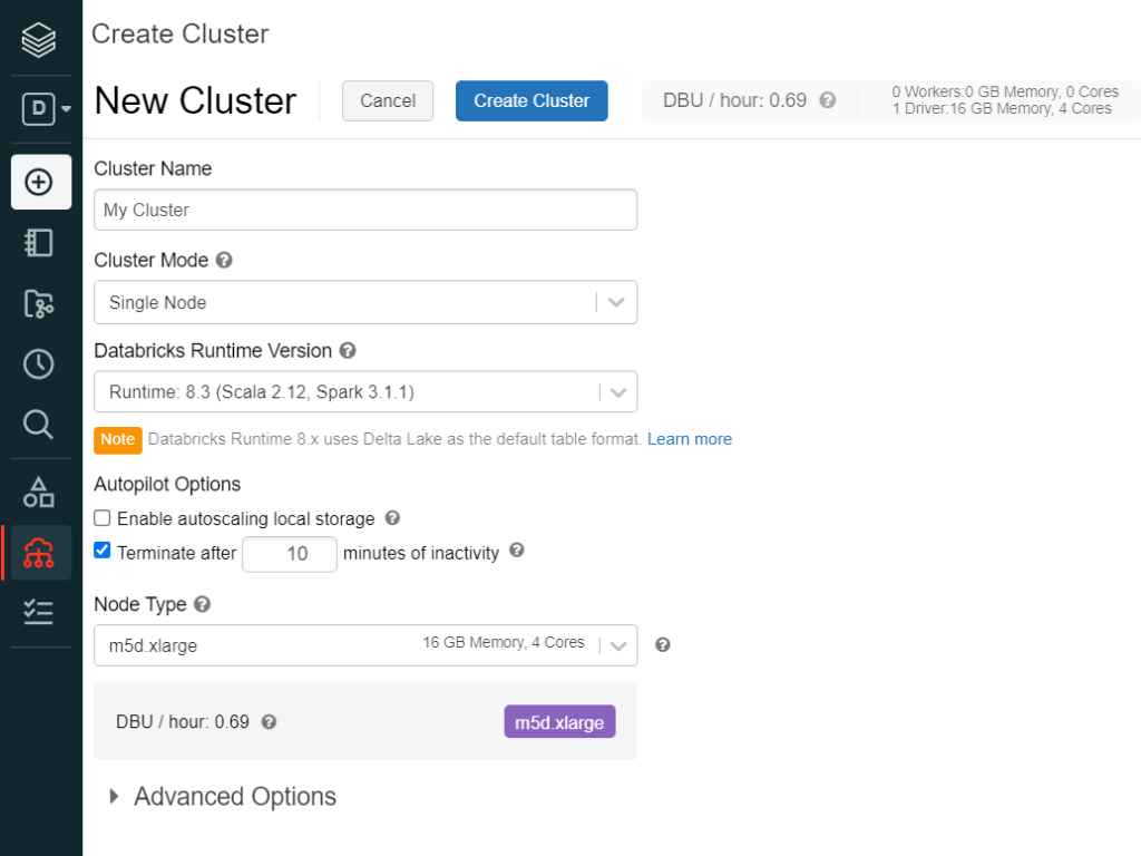
As we can see, in addition to choosing the cluster mode and the node type, Databricks clusters can be set to automatically suspend after an idle time to save unnecessary costs, as well as to automatically scale local storage, creating additional EBS (Amazon Elastic Block Storage) volumes in the user’s AWS account when needed.

Alternatively, if the cluster mode is set to Standard or High Concurrency, the minimum and maximum number of worker nodes can be selected, as well as their node type – which can be different from the driver’s.

This allows automatic adaptation to variant work volumes, in addition to helping reduce costs, as only the minimum number of clusters will be running when underloaded.

Hands-on Databricks

Having now introduced Databricks, we will use it to query data in S3, specifically the three versions of the TPC-H dataset we generated in the first blog post of this series.

In Databricks, in most cases the web-based interface is provided by Jupyter-like notebooks that contain runnable code, visualisations, and narrative text. They allow collaboration between team members, as well as history revision, and there are extra features for machine learning and job scheduling. In order to create the external tables in Databricks you need to create mounts, which are basically pointers to the S3 buckets:

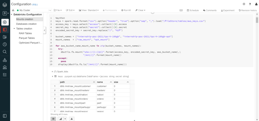
As we can observe, despite being an SQL notebook, this step was written in Python. This is another useful feature of Databricks notebooks: regardless of the notebook language, individual cells can be set to other languages.

In the image above, we can also see how Databricks automatically divides the code into Spark Jobs (seven in this specific case). Each Spark job is divided into stages, and the UI displays a progress bar to show the stage which the job is currently at. This is uncommon in querying services, but very useful as it gives the user an approximate idea of how the process is evolving, and how many tasks are missing in each stage.

Finally, this image also shows part of the results of the cell, as it displays the list of objects found in each mount. We can see how they are presented in a table format with the results as rows, but in addition to the typical CSV download, it also allows the user to see the results in a graphical view.

After creating the mounts, three databases were created, one for each version of the dataset used (CSV, Parquet, partitioned Parquet) where their respective external tables were placed:

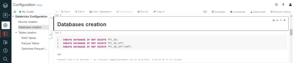
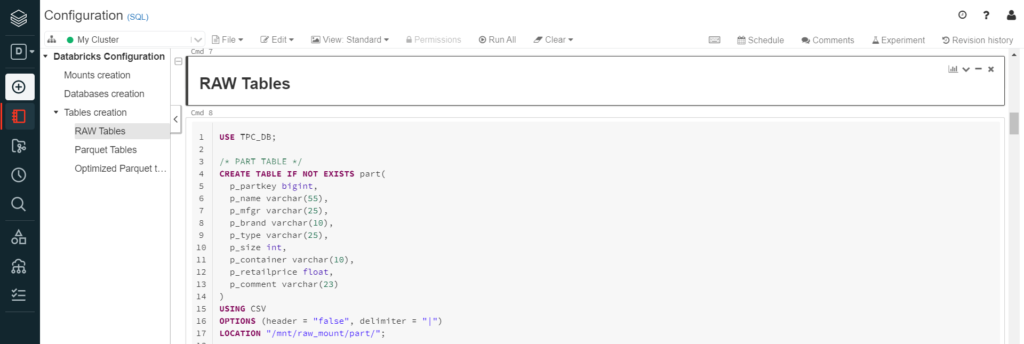
Then the external tables were created with the attribute names and their data type. The process was basically the same for the three different filetypes, only specifying the used filetype, and the compression attribute when necessary, or the different options for Parquet and CSV files:

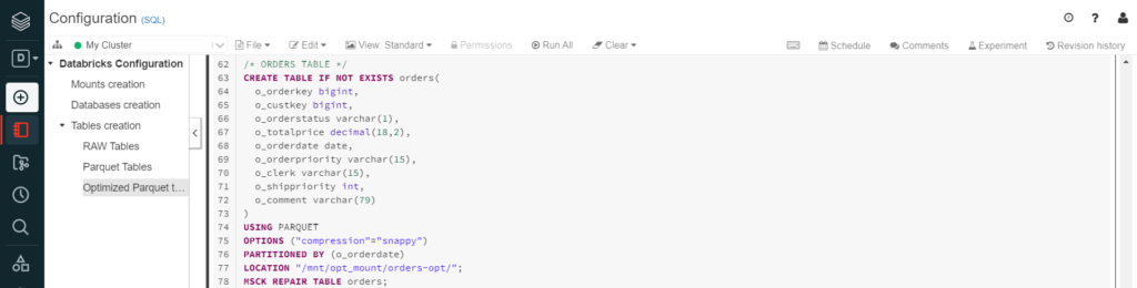
From the partitioned table, we can also see how “MSCK REPAIR TABLE” was needed in order to generate and register the table partitions in the Hive metastore. Alternatively, the function “ALTER TABLE RECOVER PARTITIONS” would perform the same job.

Once all tables had been created, we executed our ten queries for each data format, using another notebook.

First, a widget was created. Widgets are another useful Databricks utility tool, working as variables that the user can easily introduce from the main window. In addition, the notebook can be set to automatically run itself when this variable changes:

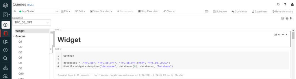
Specifically, the widget was used to display a dropdown list with the database names; just select the database from the list and all the queries begin to run:

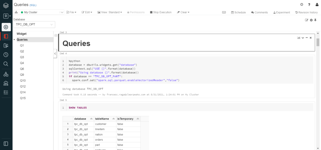
Due to an issue with different filetype attributes, the Spark configuration of the cluster had to be changed to disable the vectorised reader for the partitioned tables. Python was used to disable the option only when that specific database was selected, as we can see above.

Additionally, the tables were shown to ensure the database was correctly selected.

Finally, all the queries were executed in individual cells to show the specific elapsed time of each, as well as the individual results:

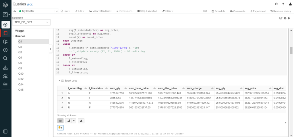
In this image, we can again see how Databricks divides the code into Spark Jobs (two in this case).

In some cases, Databricks gives tips to accelerate queries, such as to enable Delta cache, or to convert the table to Delta and optimise it in a specific column. Delta tables are Spark’s alternative to Parquet, with improved performance and data corruption prevention as their main advantages. On the other hand, Delta cache is a functionality for Parquet and Delta tables, that automatically saves the results of executed queries inside the node’s internal storage, as well as the frequently queried tables:

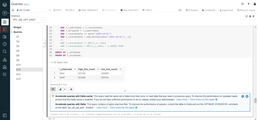
In our case, these tips were ignored, as they go beyond the scope of the project, and the queries would not be frequently executed. However, it is highly recommendable to pay attention to these recommendations if the type of query that activated them is going to be used frequently. Additionally, using Delta cache could have disabled the ability to replicate our execution times when running the same queries individually. You can find extra information on Delta in the Databricks documentation.

Results Analysis

In all cases, Databricks relied on the data lake it is querying from, in this case S3. That means that it does not store any data on its own, and the format of the data to be queried is important.

We can see how execution times are greatly reduced when changing the dataset format from CSV to Parquet, as well as how using partitioned Parquet results in faster queries in some specific cases, while maintaining or even slowing down others, mainly depending on the suitability of the partition for the specific query.

Tableau Connection

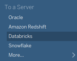
Connecting Tableau to Databricks is simple. Databricks will appear in the Connect to a Server list, and after installing the Simba Spark ODBC Driver, it will be ready to connect:

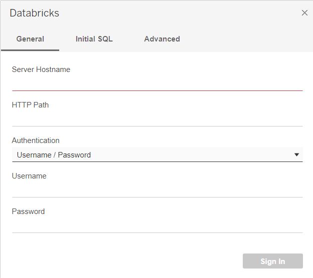
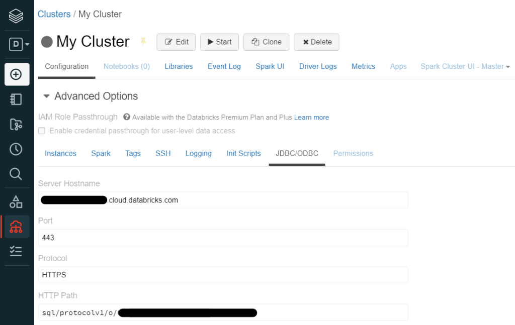
When doing so, it will ask for the server hostname (that can be identified as the URL from where the Databricks console is used) and a HTTP path. They can easily be found in the Advanced Options of the cluster in the “JDBC/ODBC” tab:

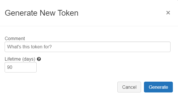
Additionally, an authentication method is required. The easiest way would be using the user and password to enter the account. Alternatively, a Personal Access Token can be provided, which can be generated in the Access Token tab of the User Settings window:

Once Databricks has been connected to Tableau, it can be used normally by selecting a database and connecting tables or using custom SQL commands, in which case do remember that the full name of the table will be needed (including the database name).

Conclusion

Databricks proved to be a well-equipped option for a data lakehouse, introducing all the benefits of warehouses on top of existing data lakes. It is easy to learn as the syntax used is like other data services based on Spark. Additionally, it incorporates Jupyter-like notebooks that allow the user to write in different programming languages (such as Scala, Python, R, or SQL) as well as introducing handy utility tools. Databricks also natively supports external tables even from partitioned files without many complications.

While Snowflake is a data warehouse that tries to incorporate analytical processes, Databricks is an analytical tool that attempts to incorporate warehouse querying capabilities. Snowflake still relies on the optimisation of its internal tables, and Databricks depends on leveraging Spark to analyse data directly in S3.

Databricks’ most important benefits are:

• Independent of the storage.
• Highly scalable compute.
• Collaborative multi-language notebooks.
• Support for most structured and semi-structured data formats.
• Pay-per-use mechanism.

While the drawbacks we found were:

• Need of external cloud provider for compute resources.
• Lack of user interface to connect data sources.
• Errors difficult to understand.
• Costs go on top of all cloud provider costs.

We can conclude that Databricks is a great option when considering a lakehouse with minimal complications to simplify the querying process, with its easy-to-write notebooks that leverage the Spark cluster.

In the upcoming blog post in this series, we are going to talk about Dremio, a data lake querying engine that differs from those we have already looked at. Dremio leverages virtualisation and caches for querying acceleration to query S3 without requiring an extra copy of the data. Stay tuned to discover how Dremio can optimise your business!

For more information on how to get the most out of Databricks, do not hesitate to contact us! We will be happy to help and guide you into taking the best decision for your business.