06 Mar 2024 Using Snowpark and Model Registry for Machine Learning – Part 1

In the dynamic data analytics landscape, the effective management of machine learning models is essential for unlocking actionable insights. Today, we’ll focus on the cutting-edge Snowpark feature, Model Registry (currently in preview), a tool that empowers Snowflake users to save and organise various trained machine learning models within a Snowflake database.

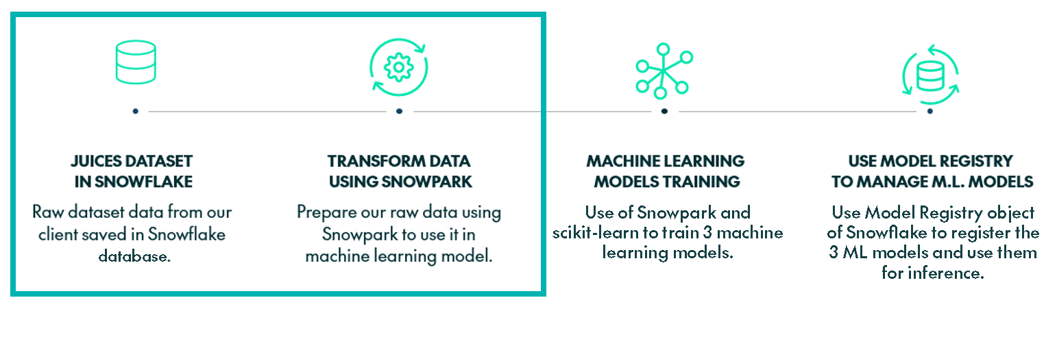
In this 2-part mini-series, we’ll guide you through the necessary steps to create a Snowpark session, perform feature engineering on a Snowpark table for data preparation, train three distinct machine learning models, and ultimately, register them in Snowflake using the new Model Registry feature. While we won’t be delving too deeply into exhaustive data preparation and model training, we will provide a clear understanding of Model Registry’s functionality and its importance in streamlining the model management process. Today, in the first part, we’ll run through all the data engineering processes, applying different packages and functions to obtain a dataset that’s ready to use for machine learning model training, which we’ll look at in the second part.

It’s worth noting that this blog post is based on insights gleaned from the amazing Snowflake hands-on sessions. In fact, certain sections of the code in this blog post may resemble the code from these sessions, which provided valuable models in constructing this guide.

The dataset we used is from this Kaggle dataset about wines, transposed to a juice factory.

Requirements

• Snowflake account with Anaconda Integration enabled by ORGADMIN
• Python 3.9
• Jupyter Notebook

Use Case Working Scenario

Imagine that we are consulting for a company in the juice manufacturing industry. Our customer, a leading juice manufacturer, has curated a comprehensive table within Snowflake named ‘JUICE_RATINGS’, encapsulating diverse ratings of their products, including detailed information such as juice type, production year, price, and intrinsic characteristics like acidity and body.

The customer wants to understand the factors behind the ratings. Does the price exert a significant influence? Do consumers lean towards juices with high or low acidity? Is there a particular type of juice that’s popular with certain customers? To answer these questions and others, the customer tasked us with a thorough machine learning study.

The dataset is in its raw form within the ‘JUICE_RATINGS’ table, housed in the ‘JUICES’ database under the ‘JUICES_DATA’ schema. Our objective is to obtain meaningful insights that will empower our customer to see what influences the ratings. The ‘rating’ within the dataset will be our target variable for study, and we’ll develop a machine learning model to predict which juices will receive favourable ratings (over 4.5 stars) and which will fall below this threshold.

Creating A Snowpark Session

Before diving into Snowpark, establishing a Jupyter environment is a prerequisite, and we guide you through the setup in our previous this Snowpark blog post. Ensure that the versions within your Jupyter environment align with those in Snowflake to mitigate potential issues, particularly when translating Python functions into stored procedures. Note that the Model Registry feature is available as of the ‘snowflake-ml-python version 1.2.0’ onwards. For this demo we used the following dependency versions; bear in mind that Jupyter environment versions must match the Snowflake Anaconda packages versions:

Dependencies:
  - python=3.9
  - pip
  - pip:
    # Snowpark
    - snowflake-snowpark-python[pandas]==1.6.1
    - snowflake-ml-python==1.2.0

    # Basics
    - pandas==1.5.3
    - numpy==1.23.5
    # ML
    - scikit-learn==1.2.2
    - lightgbm==3.3.5
    - xgboost==1.7.3
    # Visualization
    - seaborn==0.12.2
    - matplotlib==3.7.1
    # Misc
    - cloudpickle==2.0.0
    - jupyter==1.0.0
    - imbalanced-learn==0.10.1
    - anyio==3.5.0
    - typing-extensions==4.7.1  

To initiate a session with Snowpark, essential for connecting to Snowflake data, you should first understand the unique capabilities Snowpark offers for optimising your data operations, particularly in the realm of machine learning. Snowpark stands out for its adaptability in assigning roles and selecting warehouses, a feature that significantly enhances the efficiency of machine learning training processes. For example, an X-SMALL warehouse may suffice for data transformations, but for model training a larger warehouse is needed. Snowpark lets users scale their computational resources up to meet the demands of model training, providing a flexible and secure environment.

Now let’s lay the groundwork for connecting to Snowflake data via Snowpark by defining the essential parameters for the connection and specifying the warehouses required for our process:

state_dict = {
    "connection_parameters": {"user": ,
                              "account": ,
                              "role": "ACCOUNTADMIN", #OPTIONAL
                              "database":"JUICES", #OPTIONAL
                              "schema": "JUICES_DATA" #OPTIONAL
                            
                             },
    "compute_parameters" : {"default_warehouse": "XSMALL_WH",  
                            "fe_warehouse": "MEDIUM_WH",
                            "train_warehouse": "XLARGE_WH"
                            
                           }
}

# extra documentation:
# https://docs.snowflake.com/en/developer-guide/snowpark/python/creating-session
# https://docs.snowflake.com/en/developer-guide/udf/python/udf-python-packages#using-third-party-packages-from-anaconda.
# https://docs.snowflake.com/en/user-guide/admin-account-identifier

We’ll connect with our username and password and then save our connection credentials in a JSON file:

import snowflake.snowpark as snp
import json
import getpass

account_admin_password = getpass.getpass('Enter password for user with ACCOUNTADMIN role access')
 
state_dict['connection_parameters']['password'] = account_admin_password

with open('./state.json', 'w') as sdf:
    json.dump(state_dict, sdf)

Once all the connection parameters have been defined, we can start our Snowpark session. This connection establishes a link between the Snowflake account and Jupyter, enabling us to connect to our account database:

session =
snp.Session.builder.configs(state_dict["connection_parameters"]).create()

Snowpark allows us to do nearly all the operations we would perform in a Snowflake SQL session. In this case, we will create the different warehouses required for this session and grant them usage permissions for the ‘SYSADMIN’ role, responsible for executing all data transformations:

session.use_role('ACCOUNTADMIN')
project_role='SYSADMIN'

for wh in state_dict['compute_parameters'].keys():
    if wh != "train_warehouse":
        session.sql("CREATE OR REPLACE WAREHOUSE
 "+state_dict['compute_parameters'][wh]+\
                " WITH WAREHOUSE_SIZE = 
'"+state_dict['compute_parameters'][wh].split('_')[0]+\
                "' WAREHOUSE_TYPE = 'STANDARD' AUTO_SUSPEND = 60 AUTO_RESUME = 
TRUE initially_suspended = true;")\
            .collect()
    elif wh  == "train_warehouse":
        session.sql("CREATE OR REPLACE WAREHOUSE 
"+state_dict['compute_parameters'][wh]+\
                " WITH WAREHOUSE_SIZE = 
'"+state_dict['compute_parameters'][wh].split('_')[0]+\
                "' WAREHOUSE_TYPE = 'HIGH_MEMORY' MAX_CONCURRENCY_LEVEL = 1 
AUTO_SUSPEND = 60 AUTO_RESUME = TRUE initially_suspended = true;")\
            .collect()
    session.sql("GRANT USAGE ON WAREHOUSE 
"+state_dict['compute_parameters'][wh]+" TO ROLE "+project_role).collect() 
    session.sql("GRANT OPERATE ON WAREHOUSE 
"+state_dict['compute_parameters'][wh]+" TO ROLE "+project_role).collect() 
    
session.use_role(state_dict['connection_parameters']['role'])

Data Preparation

After establishing our session, the next phase involves data engineering to refine and prepare the data for machine learning model training within Snowpark. This process is streamlined thanks to Snowpark’s extensive range of functions, encompassing tasks such as adding columns, altering data types, and executing transformations. What’s more, Snowpark integrates pre-processing and imputation functions within its machine learning modelling packages, simplifying critical data engineering tasks like scaling, handling missing values, and converting categorical variables into one-hot encoding.

For the purposes of this blog post, the raw data has already been loaded into the Snowflake table called ‘JUICE_RATINGS’. For comprehensive insights into data loading using Snowpark, check out the Snowflake hands-on series. As we proceed, we will define our role (‘SYSADMIN’) and the warehouse (‘fe_warehouse’) that will be used in this part of the session:

session.use_role("SYSADMIN")
session.use_warehouse(state_dict['compute_parameters']['fe_warehouse'])

print(session.get_current_role())
print(session.get_current_warehouse())

We import all the different packages that we’ll need and load the table as a Snowpark DataFrame:

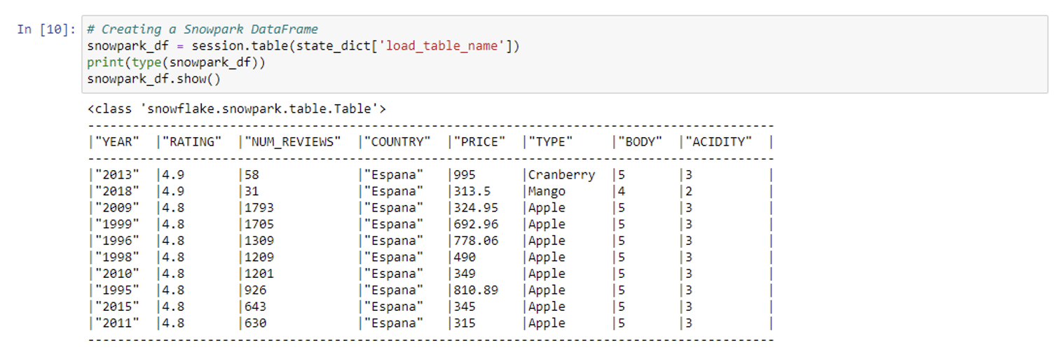
import snowflake.snowpark.functions as F
import snowflake.snowpark.types as T
from snowflake.snowpark.window import Window
from snowflake.ml.modeling.preprocessing import *
from snowflake.ml.modeling.impute import *

import sys
import json
import pandas as pd
import matplotlib.pyplot as plt
import numpy as np

# We add the table name to state_dict
state_dict['load_table_name'] = 'JUICE_RATINGS'

# Creating a Snowpark DataFrame
snowpark_df = session.table(state_dict['load_table_name'])
print(type(snowpark_df)) #Snowpark.table
snowpark_df.show() 

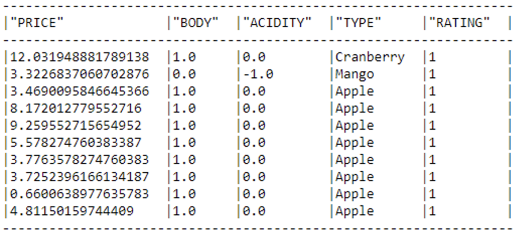
The Snowpark table will look like this:

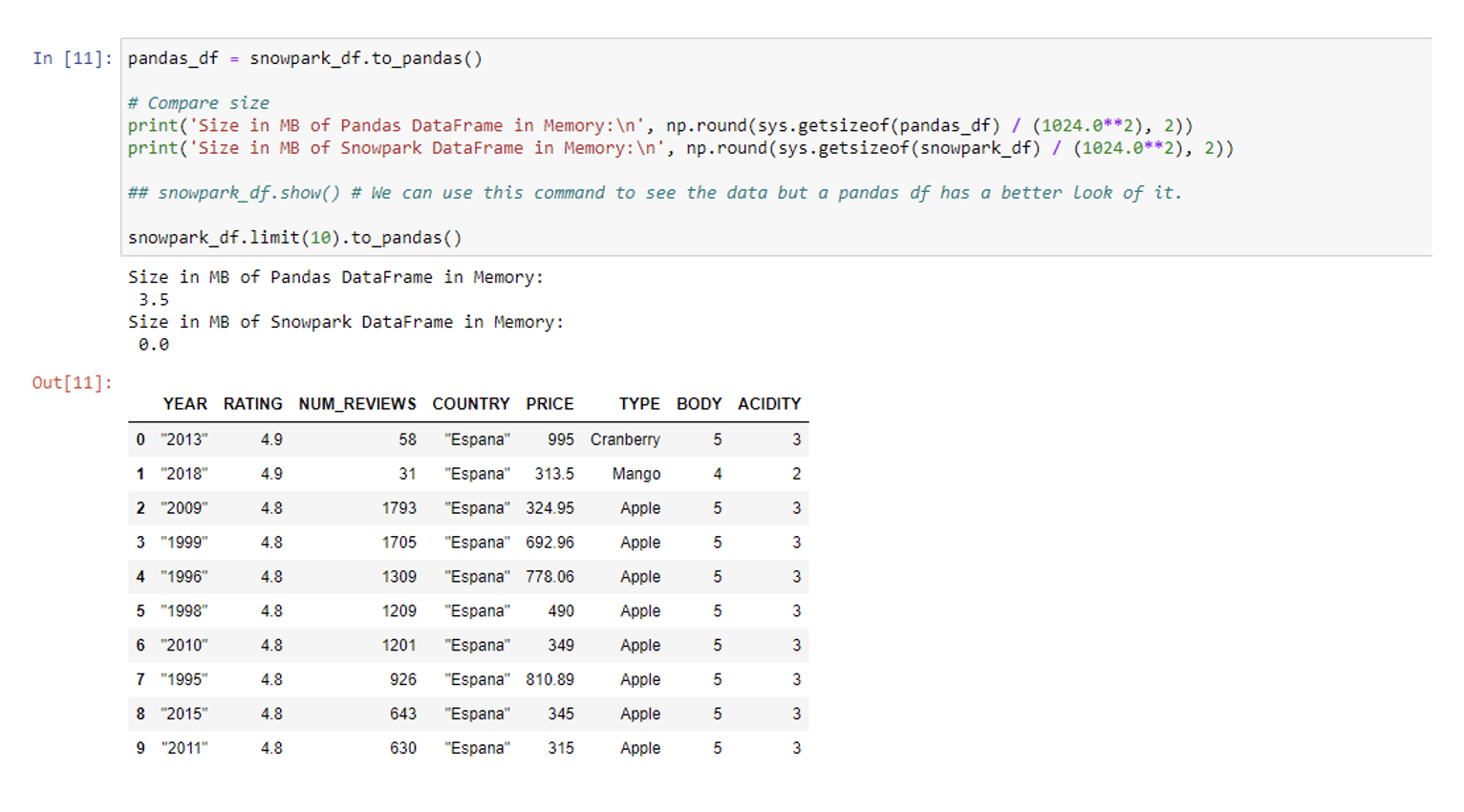
A Snowpark DataFrame can be converted into a pandas DataFrame, pulling the data from Snowflake into the Python environment memory. The only thing stored in a Snowpark DataFrame is the SQL needed to return data:

pandas_df = snowpark_df.to_pandas()

# Compare size
print('Size in MB of Pandas DataFrame in Memory:\n',
np.round(sys.getsizeof(pandas_df) / (1024.0**2), 2))
print('Size in MB of Snowpark DataFrame in Memory:\n', 
np.round(sys.getsizeof(snowpark_df) / (1024.0**2), 2))

# snowpark_df.show() # We can use this command to see the data, but it looks better in a pandas df

snowpark_df.limit(10).to_pandas()

We’ll begin by examining the structure of the table containing our raw data, as well as the number of variables and rows:

print("Number of variables:",len(snowpark_df.columns) )
print("Number of rows:",snowpark_df.count()) 

snowpark_df.schema

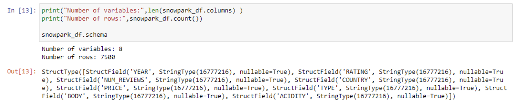
In this case, all columns are set as String type; the dataset comprises 8 variables and 7,500 rows. For this blog post, we are opting for a focused analysis, limiting our examination to specific columns. So we’ll only consider the columns ‘Price’, ‘Type’, ‘Body’, ‘Acidity’, and ‘Rating’, with the latter acting as our designated target variable to study:

snowpark_df = snowpark_df.drop('NUM_REVIEWS','YEAR','COUNTRY')
snowpark_df.limit(10).to_pandas()

Duplicate Removal

We’ll start our data transformation by checking the number of duplicated rows:

duplicates = snowpark_df.to_pandas().duplicated()
duplicates = duplicates.where(duplicates == True)

print('Number Duplicates:', duplicates.count())

We’ve identified a substantial count of 5,549 duplicated values, and in a real-world scenario we’d have to assess the viability of continuing with such a dataset. However, for the purposes of this demonstration, we’ll keep using it, eliminating the duplicates to enhance the dataset’s reliability and integrity for subsequent analysis:

snowpark_df = snowpark_df.drop_duplicates()
snowpark_df.count()

Now our table has 1,951 rows.

Transformation of Our Target Variable – ‘Rating’

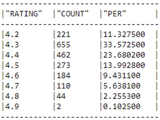
We are now ready to adjust our target variable, ‘Rating’, to meet the customer’s requirements. As mentioned previously, our objective is to determine which juices have favourable ratings (equal to or exceeding 4.5) and which don’t (under 4.5). Our initial focus will be centred on examining the proportions within our target data:

tot = snowpark_df.count()
snowpark_df.group_by('RATING').count().sort('RATING')\
                        .with_column('PER',F.col('COUNT')/tot*100)\
                        .show()

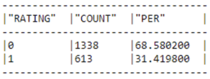
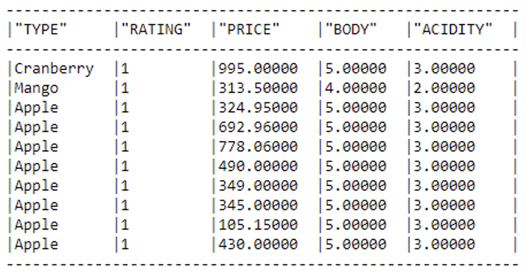
Our next task involves categorising the varied ratings, in line with the customer’s specific demands: all ratings below 4.5 will be categorised as ‘BAD’ (labelled as 0), whilst those equal to or exceeding this threshold will be designated as ‘GOOD’ (labelled as 1):

snowpark_df = 
snowpark_df.with_column('RATING',F.iff(F.col('RATING').in_(['4.5','4.6','4.7','4.8','4.9','5']), 1, 0))

snowpark_df.group_by('RATING').count().sort('RATING')\
                        .with_column('PER',F.col('COUNT')/tot*100)\
                        .show()

Now our target variable looks like this:

Datatype Transformation and Missing Values Imputation

We’ll now convert the numerical variables (‘Price’, ‘Body’, and ‘Acidity’) from strings to numerical types and evaluate the need for imputing N.A. values:

number_col = ['PRICE','BODY','ACIDITY']

snowpark_df =  snowpark_df.replace("NA",None) #Replace NA string by None values

#Lets transform to numeric values
for column in number_col:
    snowpark_df = snowpark_df.withColumn(column,F.to_decimal(column,38,2))

snowpark_df.group_by('BODY').count().show()

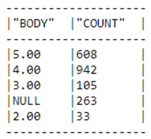
As we can see, there are null values in the ‘Body’ and ‘Acidity’ columns. For the sake of expediency, we’ll take a straightforward approach to handling these null values by replacing them with the mean of their respective columns:

for column in number_col:
    snowpark_df = 
snowpark_df.withColumn(column,F.iff(F.col(column).is_null(),F.avg(F.col(column)).over(),F.col(column))) 

snowpark_df.show()

Scaling the Numerical Variables

As we said before, Snowpark can use different data pre-processing functions: one of these functionalities is ‘RobustScaler’, which enhances the dataset’s numerical features, optimising their scale for improved model training efficiency:

my_scaler = RobustScaler(input_cols=number_col, output_cols=number_col)
my_scaler.fit(snowpark_df)
snowpark_df = my_scaler.transform(snowpark_df)

snowpark_df.show()

One-Hot Encoding on Categorical Variables

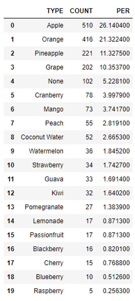
We are now set to transform and categorise the ‘Type’ variable into One-Hot Encoding columns using Snowpark. The first step is to examine the proportions of this variable:

snowpark_df.group_by('TYPE').count().sort(F.col('COUNT').desc())\
                        .with_column('PER',F.col('COUNT')/tot*100)\
                        .to_pandas()

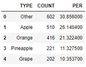
We will transform the data by consolidating all values that account for less than 10% into a single category labelled ‘Others’. Although this approach might not be the most suitable for this specific dataset, we’ll do it for the purposes of this example. This strategic adjustment leads to a more streamlined representation of the ‘Type’ variable:

Type_keep = ["Apple","Orange","Pineapple","Grape"]

# We remove the "" from the name and then we change the type keep to other 
snowpark_df =snowpark_df.with_column('TYPE',F.iff(F.col('TYPE').in_(Type_keep), F.col('TYPE'), "Other"))



snowpark_df.group_by('TYPE').count().sort(F.col('COUNT').desc())\
                        .with_column('PER',F.col('COUNT')/tot*100)\
                        .to_pandas()

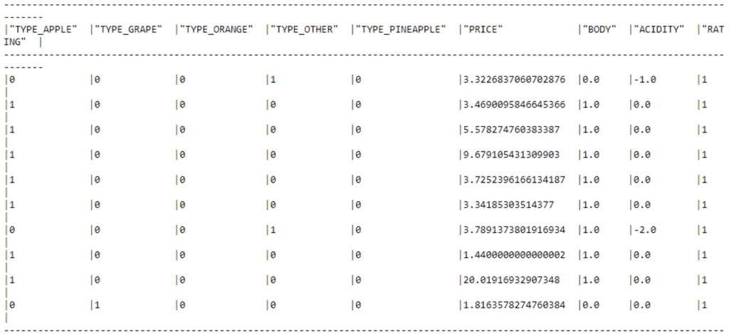
Now we can convert the variable into One-Hot Encoding columns:

# Prepare values for One-Hot-Encoding
ohe_cols = ['TYPE']

def fix_values(columnn):
    return F.upper(F.regexp_replace(F.col(columnn), '[^a-zA-Z0-9]+', '_'))

for col in ohe_cols:
    snowpark_df = snowpark_df.with_column(col, fix_values(col))

my_ohe_encoder = OneHotEncoder(input_cols=ohe_cols, output_cols=ohe_cols, drop_input_cols=True)
my_ohe_encoder.fit(snowpark_df)
snowpark_df = my_ohe_encoder.transform(snowpark_df)
snowpark_df.show()

And at last, the data is ready for machine learning training! Let’s save the refined table in our Snowflake database:

snowpark_df.write.save_as_table(table_name='JUICES_PREPARED', mode='overwrite')

Conclusions & What’s Next

Snowpark proves itself to be a formidable platform that empowers data professionals with a wide range of capabilities for efficient data transformation. Its robust features, ranging from basic tasks like type conversion to more advanced operations such as duplicate removal and One-Hot Encoding, guarantee its versatility and efficiency in preparing data for machine learning model training. Moreover, Snowpark’s flawless integration with the versatile Snowflake platform, encompassing the creation of various roles and warehouses, further enhances its appeal as a comprehensive solution for data management and analysis within the Snowflake ecosystem.

What’s more, the availability of various packages to extend Snowpark’s capabilities offers us even more possibilities: through integration with external libraries such as scikit-learn, Snowpark allows data scientists to effortlessly incorporate their preferred tools and techniques, promoting innovation and accelerating the development of machine learning models. As organisations increasingly leverage data-driven insights, Snowpark stands out as a vital component of their toolkit, allowing teams to unlock the full potential of their data assets whilst ensuring agility and scalability in their analytical workflows.

Don’t miss the next part of the series where we will explore machine learning model training and the amazing Model Registry feature for ML model management! In the meantime, don’t hesitate to contact us if you have any questions or need further information – our team is ready to provide the support you need to make the most of your data science journey.